I’ve been working on camera and lens simulation for a couple of weeks, and I decided that I needed a technique for calculating the spatial frequency responses (SFRs) and modulation transfer functions (MTFs) of synthetic images that was a) completely open, so I could understand just what it was doing, and b) embeddable in my Matlab simulator, so that I could automate the generation and analysis of MTFs.
It turns out that when the ISO 12233 target was updated in the middle of the last decade, Peter Burns wrote a Matlab program to do spatial frequency analysis of slanted edge targets. He continued to update it, and the latest version, sfrmat3, is available for download here. The program can operate as a Matlab function with no user input, or it can use a GUI to allow the user to specify a file and a region of interest (ROI) for the SFR analysis. I’m using it without the GUI, since one of the things I’m trying to do is automate the analysis.
The Burns code was the starting place for Imatest, but they have made what they consider to be – and probably are – improvements over the years, and those improvements are proprietary. Sfrmat3 is source code; if you want to see what it’s doing, you can just look.
The first thing I did after I got the Burns’ code integrated with mine was plot the MTF of a Bayer-CFA camera with a 4.77 um pixel pitch (like the Sony a7R or the Nikon D800), and 100% fill factor. I used 650 nm red light, 550 nm green light, and 450 nm blue light to compute the lens diffraction. This is a 14-bit camera, and has no noise except the quantization noise of the (perfect, of course) analog-to-digital converter (ADC). I demosaiced the RGGB captured image with bilinear interpolation, then measured and plotted the luminance MTF. Here’s what I got, with the MTF plotted against cycles/pixel:
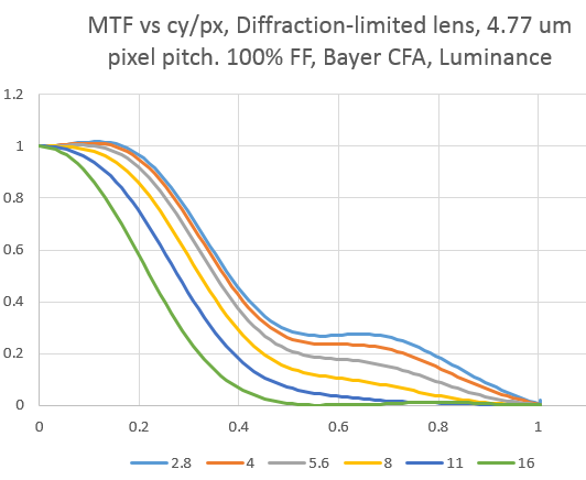
Spatial frequency information of over ½ cycles per pixel is aliased upon reconstruction, and there is quite a bit of it at wider f-stops.
Most sampling theory starts with what’s called a point sampler, a Platonic ideal of a sensor that samples the scene with a grid of infinitely-small points. I set the fill factor of the simulated camera to 1% to get an idea of what things would be like as the camera’s sensels headed in that direction:
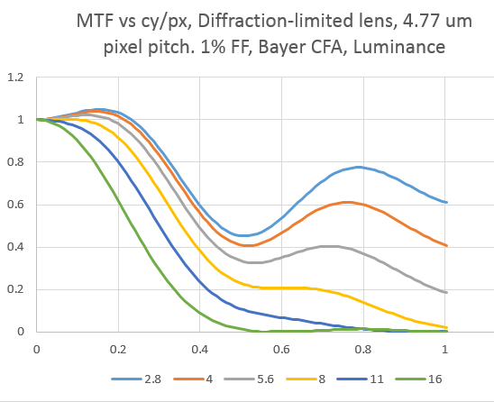
There is an awful lot of energy above half the sampling frequency. From the point of view of aliasing, it’s a good thing that modern sensors, especially ones with micro-lenses, have fill factors that can approach one. Note that the small sampling area does improve sharpness at frequencies below half a cycle per pixel.
If you want to see what that much aliasing looks like, here’s a close-up:

For my next simulation run, I set the fill factor to 400%. This gives us a special kind of anti-aliasing filter, since each sensel gathers light from an area that encompasses half the area of the four adjacent sensels, and a quarter the area of the diagonally-adjacent sensels. Here’s what the MTF for that camera looks like:
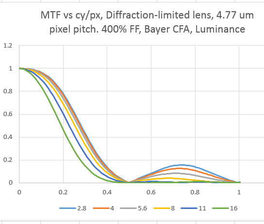
You can see that this kind of AA filter is very good at reducing the amount of energy close to half the sampling frequency without affecting the spatial frequencies below that as badly as stopping down the lens far enough to produce zero energy at ½ a cycle per pixel. However, when we stop down the lens, the energy doesn’t bounce back between 0.5 cycles/pixel and 1 cycle/pixel, which is what happens with this kind of AA filter.
Most lenses are not diffraction-limited, at least at some apertures. There are many sources of blur. Some have approximated blur by repeated applications of a pillbox (constant, circular) convolution kernel. Many applications of that kernel result in the same result that applying a Gaussian kernel once would give. I applied a one-pixel radius pillbox kernel twice to the target, in addition to the diffraction simulation. Here’s what resulted:
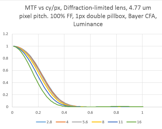
You can see that this is very effective in removing energy in the region between 0.5 and 1.0 cycles/pixel. It does affect the diffraction-limited response at the wider f-stops quite a bit, essentially removing any improvement in resolution stemming from opening up the lens after f/5.6.
It is instructive to compare the MTFs of a f/2.8 lens and a 1 pixel double pillbox with a simple f/16 diffraction limited lens:
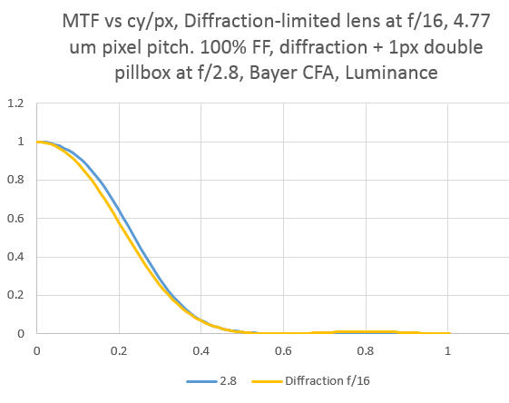
You’re better off with the double pillbox. To the extent that the double pillbox is a good model for slight defocusing, that could be slightly better, but harder to control, strategy to avoid aliasing then diffraction. It’s so hard to control that I’m pretty sure this information is only of academic use.
Hi Jim, moving right along I see 🙂
FYI the 4-dot beam splitting AA that appears to be part of recent Nikon cameras tends to apply a shift of +/- 0.35-0.4 pixels laterally and vertically with respect to the center of a pixel, so 400% FF seems like overkill for those (see this post by Frans van den Bergh for more http://mtfmapper.blogspot.it/2012/06/nikon-d40-and-d7000-aa-filter-mtf.html?showComment=1350226688984#c2356900874820952362)
Also, I do not recognize the larger aperture shapes shown in your top graph above Nyquist from any real life MTF curve measurement I have seen (although I normally work on raw data). I’ll have to try a couple of examples with bicubic to see whether it can cause that.
Jack
Jack, thanks for the link. I’ll check it out. Also, you probably won’t see curves like the large-aperture ones any time soon, diffraction-limited f/2.8 DSLR lenses being pretty thin on the ground.
Of course, I could have a bug in the code…
Good point about diffraction limited f/2.8 lenses, Jim. Though most f/5.6s I have seen do not seem to be able to pull that MTF20 hovering act around Nyquist 😉
Even the Otus doesn’t look like it’s diffraction limited until about f/11.