• site home
  • blog home
  • galleries
  • contact
  • underwater
  • the bleeding edge

the last word

Photography meets digital computer technology. Photography wins -- most of the time.

You are here: Home / The Last Word / Noise reduction with nonlinear tools and downsampling

Noise reduction with nonlinear tools and downsampling

September 30, 2014 JimK 1 Comment

In the last half-dozen posts, I’ve explored the noise reduction effects and quality of the results from six or seven different downsampling methods. From doing that work, I’ve concluded that there are several choices for someone with a small-pixel camera to produce images that have similar noise characteristics as those made with a large-pixel camera, after the small-pixel images are down res’d to the resolution of the large-pixel camera, as stated by photographic equivalence.

The above depends on the FWC of the cameras being proportional to the square of the pixel pitch. It further depends on an assumption about read noise. If the read noise of the cameras involved is proportional to the pixel area, then the sun and moon align and the noise part of equivalence is handled.

But the above assumption about read noise is suspect. I’ll make one that’s pretty far out in the other direction. Let’s assume the read noise is independent of pixel size. That gives a real advantage to the large pixel cameras. Is it enough for them to win the noise battle with their small-pixel brethren at the same downsampled resolution?

Not if you throw non-linear noise reduction techniques like those baked into Lightroom and Adobe Camera Raw.

Here’s how I know. I used my camera simulator to make two “photographs” of Bruce Lindbloom’s desk, with the sim set to ISO 3200, with a 1.25 micrometer (um) pixel pitch, and a 5 um pixel pitch.

The other important parameters that I used are:

  • Simulated Otus 55mm f/1.4 lens
  • Aperture: f/5.6
  • Bayer CFA with sRGB filter characteristics
  • Fill factor = 1.0
  • 0.375 pixel phase-shift AA filter
  • Diffraction calculated at 450nm for blue plane, 550nm for the green plane, and 650nm for the red plane
  • Full well capacity = 1600 electrons per square um
  • Read noise sigma = 1.5 electrons
  •  Bilinear interpolation demosaicing

The first two images have been enlarged 3x using nearest neighbor before being JPEG’d. The second two are enlarged by 9x using the same method.

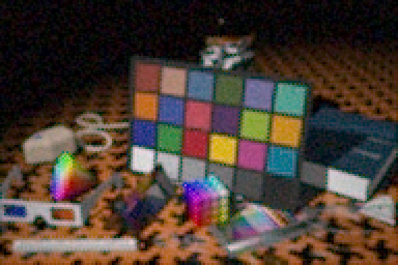
Here’s the scene as captured by the camera above with the pixel pitch set to 5 um:

LindbloomAAISO3200Pitch5-3x

And at 1.25 um, processed in Lr with luminance noise reduction set to 100, chroma noise reduction set to 100, and exported at 25% magnification by Lightroom with no sharpening:

LindbloomAAISO3200Pitch133xLrNR

Now let’s zoom in:

With the 5 um camera:

LindbloomAAISO3200Pitch59x

And the 1.25 um camera:

LindbloomAAISO3200Pitch13k9xLrNR


Being able to use nonlinear noise reduction on the higher resolution camera is a game-changer. The noise in the lower image is actually lower than that in the upper one. However, there’s much more detail in the lower image. The ugly zipper artifacts from the demosaicing are completely gone.

What if we try to do some nonlinear noise reduction on the image from the big-pixel camera. Here’s one attempt:

Lindx9AAISO3200Pitch545pctmedian

We lose sharpness and still can’t get the noise down to where it is in the 1.25 um image. We still have residual zipper artifacts on the bottom of the yellow Macbeth patch. There are color errors on the sides of the gray patches.

And this was after making some assumptions about read noise that stacked the deck in favor of the big-pixel camera.


The Last Word

← Noise performance of downsampling with eliptical weighted averaging Do color space conversions degrade image quality? →

Comments

  1. Jack Hogan says

    October 1, 2014 at 1:40 am

    Funny how the noise reduced 1.25um image appears to also have lost contrast and saturation compared to the 5um.

    Reply

Leave a Reply Cancel reply

Your email address will not be published. Required fields are marked *

May 2025
S M T W T F S
 123
45678910
11121314151617
18192021222324
25262728293031
« Apr    

Articles

  • About
    • Patents and papers about color
    • Who am I?
  • How to…
    • Backing up photographic images
    • How to change email providers
    • How to shoot slanted edge images for me
  • Lens screening testing
    • Equipment and Software
    • Examples
      • Bad and OK 200-600 at 600
      • Excellent 180-400 zoom
      • Fair 14-30mm zoom
      • Good 100-200 mm MF zoom
      • Good 100-400 zoom
      • Good 100mm lens on P1 P45+
      • Good 120mm MF lens
      • Good 18mm FF lens
      • Good 24-105 mm FF lens
      • Good 24-70 FF zoom
      • Good 35 mm FF lens
      • Good 35-70 MF lens
      • Good 60 mm lens on IQ3-100
      • Good 63 mm MF lens
      • Good 65 mm FF lens
      • Good 85 mm FF lens
      • Good and bad 25mm FF lenses
      • Good zoom at 24 mm
      • Marginal 18mm lens
      • Marginal 35mm FF lens
      • Mildly problematic 55 mm FF lens
      • OK 16-35mm zoom
      • OK 60mm lens on P1 P45+
      • OK Sony 600mm f/4
      • Pretty good 16-35 FF zoom
      • Pretty good 90mm FF lens
      • Problematic 400 mm FF lens
      • Tilted 20 mm f/1.8 FF lens
      • Tilted 30 mm MF lens
      • Tilted 50 mm FF lens
      • Two 15mm FF lenses
    • Found a problem – now what?
    • Goals for this test
    • Minimum target distances
      • MFT
      • APS-C
      • Full frame
      • Small medium format
    • Printable Siemens Star targets
    • Target size on sensor
      • MFT
      • APS-C
      • Full frame
      • Small medium format
    • Test instructions — postproduction
    • Test instructions — reading the images
    • Test instructions – capture
    • Theory of the test
    • What’s wrong with conventional lens screening?
  • Previsualization heresy
  • Privacy Policy
  • Recommended photographic web sites
  • Using in-camera histograms for ETTR
    • Acknowledgments
    • Why ETTR?
    • Normal in-camera histograms
    • Image processing for in-camera histograms
    • Making the in-camera histogram closely represent the raw histogram
    • Shortcuts to UniWB
    • Preparing for monitor-based UniWB
    • A one-step UniWB procedure
    • The math behind the one-step method
    • Iteration using Newton’s Method

Category List

Recent Comments

  • bob lozano on The 16-Bit Fallacy: Why More Isn’t Always Better in Medium Format Cameras
  • JimK on Goldilocks and the three flashes
  • DC Wedding Photographer on Goldilocks and the three flashes
  • Wedding Photographer in DC on The 16-Bit Fallacy: Why More Isn’t Always Better in Medium Format Cameras
  • JimK on Fujifilm GFX 100S II precision
  • Renjie Zhu on Fujifilm GFX 100S II precision
  • JimK on Fuji 20-35/4 landscape field curvature at 23mm vs 23/4 GF
  • Ivo de Man on Fuji 20-35/4 landscape field curvature at 23mm vs 23/4 GF
  • JimK on Fuji 20-35/4 landscape field curvature at 23mm vs 23/4 GF
  • JimK on Fuji 20-35/4 landscape field curvature at 23mm vs 23/4 GF

Archives

Copyright © 2025 · Daily Dish Pro On Genesis Framework · WordPress · Log in

Unless otherwise noted, all images copyright Jim Kasson.