• site home
  • blog home
  • galleries
  • contact
  • underwater
  • the bleeding edge

the last word

Photography meets digital computer technology. Photography wins -- most of the time.

You are here: Home / Z50 / Nikon Z50 RN, FWC, and PDR

Nikon Z50 RN, FWC, and PDR

November 14, 2019 JimK 3 Comments

This is the sixth in a series of posts on the Nikon Z50. You should be able to find all the posts about that camera in the Category List on the right sidebar, below the Articles widget. There’s a drop-down menu there that you can use to get to all the posts in this series; just look for “Z50”.

Quite an alphabet soup in the title, huh? This afternoon, I ran a photon transfer curve (PTC) for the Z50, which allows me to calculate the input-referred read noise (RN) in electrons, the full well capacity (FWC), and the photographic dynamic range. Not that it matters, but I used a CV 125 mm f/2.5 Macro-Apo-Lanthar with the FTZ adapter for this job. The legendary sharpness of the lens didn’t matter much, since I defocused heavily.

First up, a set of normalized photon transfer curves:

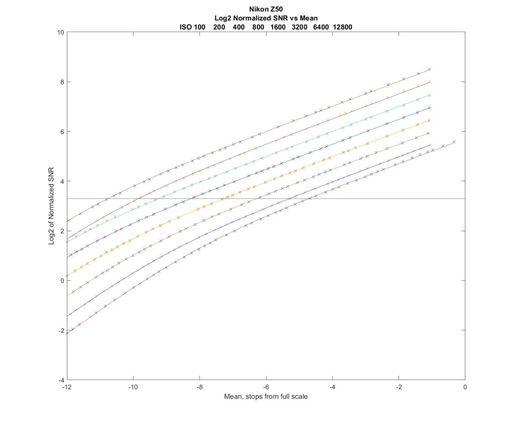
The mean signal level, in stops from full scale, is the x-axis. The y-axis is the signal to noise ratio, normalized to an 8-inch print viewed from 18 inches away using the same methodology that Bill Claff uses for his PDR measurements. The top curve is from ISO 100, the next for ISO 200, and so on. The measured data points are the crosses, and the modeled approximation is the solid lines. There is excellent agreement. Don’t worry about the solid black horizontal line for now; we;ll get to that at the end of the post.

There are two interesting things about the curve set. The first is the high shadow SNR at ISO 400. The Z50 changes to higher conversion gain at that ISO, which makes the read noise drop, and that makes the shadows less noisy. The second is the closeness of the bottom curve to the one immediately above it. That occurs because Nikon performs some noise reduction using digital signal processing at that ISO setting.

The modeler program that I wrote tell me what the full well capacity it found for each ISO setting and each raw plane. Here’s what that looks like:

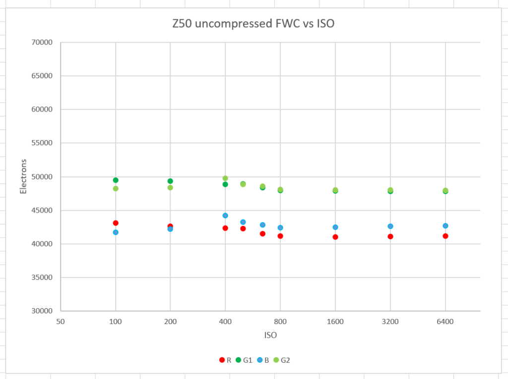
In a perfect world, all the FWCs would be the same. Here they come very close to that, for each channel considered separately. However, the red and blue channels are lower than the others. That’s due to the Nikon white balance prescaling, which confuses the software that I wrote. I have a way to calibrate out the effect, but I didn’t use it on this data set, because it requires that I figure out the gain settings for my particular serial number. Just think of the red and blue FWCs as too low, and the FWC of the camera as about 48,000 electrons.

Knowing the FWC, I can calculate the input referred read noise:

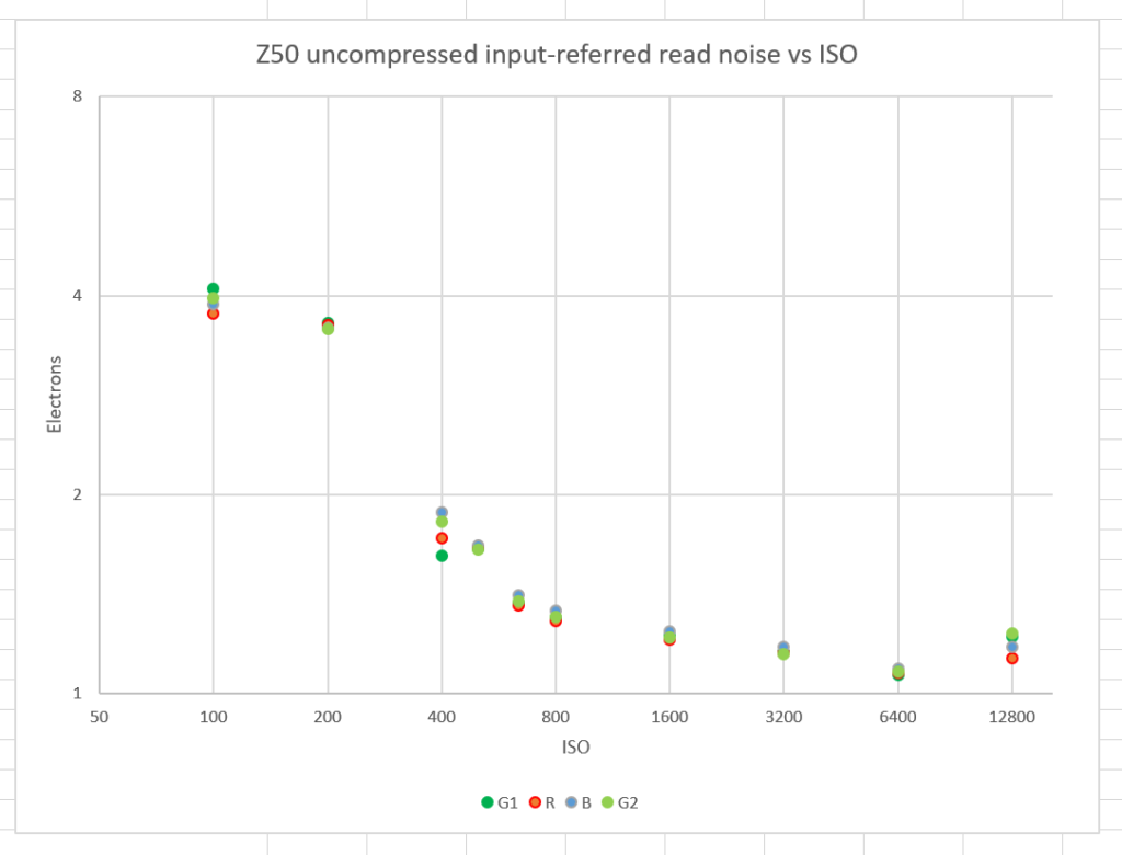
The jump downwards at ISO 400 is because of the increased conversion gain at that ISO. RN at high ISOs is approaching 1 electron, which is about the state of the consumer camera art these days.

To show you the photographic dynamic range, I’ll change the axes of the top curve in this post:

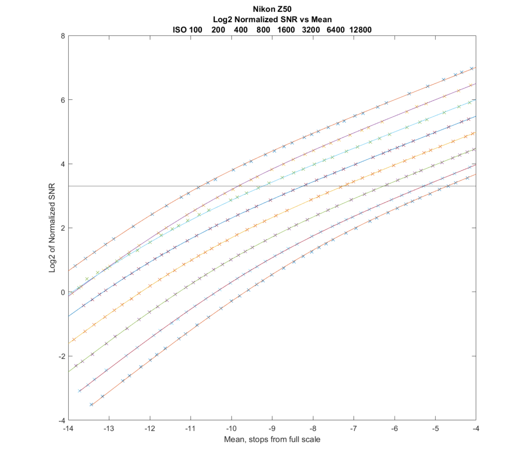
This shows the shadow signal to noise ratio as a function of ISO setting and mean signal level. The Claff PDF threshold is plotted as the black horizontal line. You can see that the PDR at base ISO is a bit over 11 stops.

This is a fine example of a typical CMOS sensor in today’s cameras. It looks like there were no compromises in IQ when this sensor was designed, even though it is used in an inexpensive camera.


Z50

← Nikon 16-50/3.5-6.3 on Z50 at 16 mm Nikon Z50 PDAF banding →

Comments

  1. Jack Hogan says

    November 14, 2019 at 11:52 pm

    A beautiful looking sensor, thanks Jim. Given the MP and elegant results, can we assume that it is a sibling of the D5/D500 sensor, supposedly designed/ manufactured by Nikon?

    Reply
    • JimK says

      November 15, 2019 at 6:44 am

      The PTCs don’t look anything like those of the D5. I haven’t tested the D500.

      Reply
    • N/A says

      November 16, 2019 at 7:10 am

      > D5/D500 sensor

      those are totally differently designed sensors ! while APS-C D500 looks exactly like Sony designs (for everybody, including Nikon) based on Aptina’s dual gain sensel architecture FF D5 looks like exactly what Sony never designs…

      http://www.photonstophotos.net/Charts/PDR.htm#Nikon%20D5,Nikon%20D500

      Reply

Leave a Reply Cancel reply

Your email address will not be published. Required fields are marked *

May 2025
S M T W T F S
 123
45678910
11121314151617
18192021222324
25262728293031
« Apr    

Articles

  • About
    • Patents and papers about color
    • Who am I?
  • How to…
    • Backing up photographic images
    • How to change email providers
    • How to shoot slanted edge images for me
  • Lens screening testing
    • Equipment and Software
    • Examples
      • Bad and OK 200-600 at 600
      • Excellent 180-400 zoom
      • Fair 14-30mm zoom
      • Good 100-200 mm MF zoom
      • Good 100-400 zoom
      • Good 100mm lens on P1 P45+
      • Good 120mm MF lens
      • Good 18mm FF lens
      • Good 24-105 mm FF lens
      • Good 24-70 FF zoom
      • Good 35 mm FF lens
      • Good 35-70 MF lens
      • Good 60 mm lens on IQ3-100
      • Good 63 mm MF lens
      • Good 65 mm FF lens
      • Good 85 mm FF lens
      • Good and bad 25mm FF lenses
      • Good zoom at 24 mm
      • Marginal 18mm lens
      • Marginal 35mm FF lens
      • Mildly problematic 55 mm FF lens
      • OK 16-35mm zoom
      • OK 60mm lens on P1 P45+
      • OK Sony 600mm f/4
      • Pretty good 16-35 FF zoom
      • Pretty good 90mm FF lens
      • Problematic 400 mm FF lens
      • Tilted 20 mm f/1.8 FF lens
      • Tilted 30 mm MF lens
      • Tilted 50 mm FF lens
      • Two 15mm FF lenses
    • Found a problem – now what?
    • Goals for this test
    • Minimum target distances
      • MFT
      • APS-C
      • Full frame
      • Small medium format
    • Printable Siemens Star targets
    • Target size on sensor
      • MFT
      • APS-C
      • Full frame
      • Small medium format
    • Test instructions — postproduction
    • Test instructions — reading the images
    • Test instructions – capture
    • Theory of the test
    • What’s wrong with conventional lens screening?
  • Previsualization heresy
  • Privacy Policy
  • Recommended photographic web sites
  • Using in-camera histograms for ETTR
    • Acknowledgments
    • Why ETTR?
    • Normal in-camera histograms
    • Image processing for in-camera histograms
    • Making the in-camera histogram closely represent the raw histogram
    • Shortcuts to UniWB
    • Preparing for monitor-based UniWB
    • A one-step UniWB procedure
    • The math behind the one-step method
    • Iteration using Newton’s Method

Category List

Recent Comments

  • JimK on Goldilocks and the three flashes
  • DC Wedding Photographer on Goldilocks and the three flashes
  • Wedding Photographer in DC on The 16-Bit Fallacy: Why More Isn’t Always Better in Medium Format Cameras
  • JimK on Fujifilm GFX 100S II precision
  • Renjie Zhu on Fujifilm GFX 100S II precision
  • JimK on Fuji 20-35/4 landscape field curvature at 23mm vs 23/4 GF
  • Ivo de Man on Fuji 20-35/4 landscape field curvature at 23mm vs 23/4 GF
  • JimK on Fuji 20-35/4 landscape field curvature at 23mm vs 23/4 GF
  • JimK on Fuji 20-35/4 landscape field curvature at 23mm vs 23/4 GF
  • Ivo de Man on Fuji 20-35/4 landscape field curvature at 23mm vs 23/4 GF

Archives

Copyright © 2025 · Daily Dish Pro On Genesis Framework · WordPress · Log in

Unless otherwise noted, all images copyright Jim Kasson.