This is the 13th in a series of posts on the Sony a9. The series starts here.
I present today a guest post from a expert (and he is one, despite his protestations below) who has helped me solve camera puzzles over the years. Take it away, Horshack.
Jim Kasson and Bill Claff have been busy trying to get to the bottom of some irregularities in their A9 sensor noise measurements. Those guys possess a deep understanding of sensor operation and measurement and so have been approaching the problem with their usual high-level, math-based theoretical analysis. Me, I’m just a data grunt with an antagonistic relationship with math – I instead like to stare at data to try and divine patterns, then come up with zany experiments to crack open engineering mysteries from the bottom-up. Experience has taught me the best way to do that is to focus on the data that’s misbehaving the most.
Jim outlined the kinks in the A9 noise measurements. The data point that’s most alluring to me is the ISO 160 -> 200 transition, specifically for the red channel. Here is a rawshack analysis of Jim’s A9 blackframes.
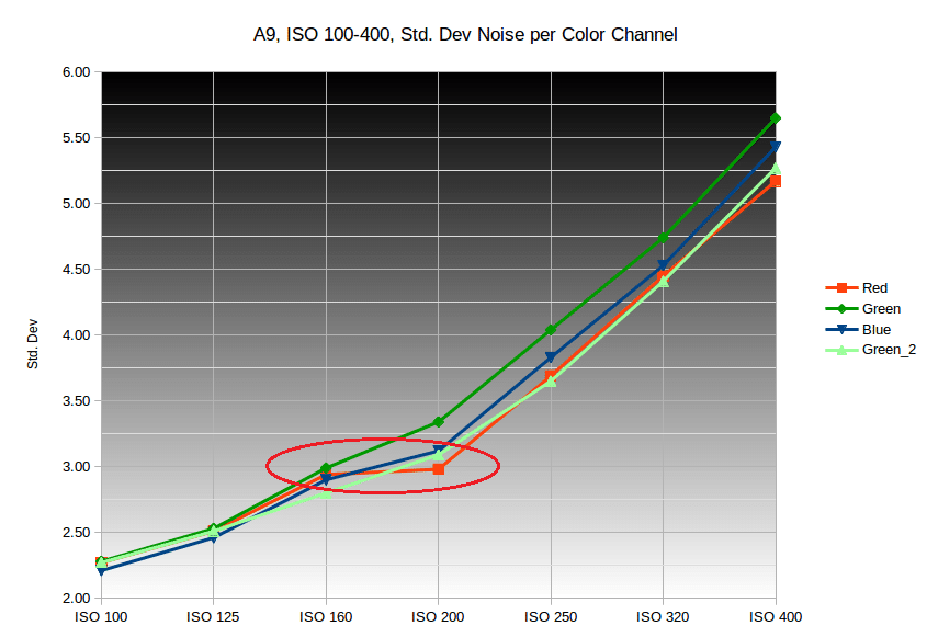
The stddev of noise for the red channel goes from 2.94 (ISO 160) to 2.98 (ISO 200). In other words, it doesn’t really go up at all. That’s not supposed to ‘not’ happen. The other channels for this ISO transition don’t go up “enough” either – look at the ISO 200 -> 250 and beyond to see what the curve is supposed to look like. But it’s the red channel that’s misbehaving the most, so that’s what we’ll focus on.
I wanted to dive into this anomaly further, so I charted the the distribution of noise on the red channel to see if it reveals anything.

This chart shows the number of pixels at each ADU value for ISOs 100-250 for blackframes. The bell-curve shape is due to the gaussian distribution of read noise. The taller and skinnier the curve, the lower the distribution, meaning less noise. Notice how the pixel count peaks at 512 – that is the defined blackpoint of the A9 sensor. Notice also that although the pixel count peaks at 512, the actual median for ISO 100 and 125 is somewhere between 510 and 512 – there are many more pixels at ADU 510/511 as there are on the opposite side of the curve at ADU 513/514. I believe this is quantization error from the ADC, although Jim can chime in to confirm. By ISO 250 the distribution across the 512 blackpoint becomes more even. What I wanted to reveal is any unusual distribution between ISO 160 and 200 since that is the misbehaving data point we’re focusing on. The distribution looks about normal. One oddity though – the pixel count @ ADU 513 is identical between ISO 160 and 200, at 786,369 pixels. Likely just very lucky random chance, but also more indication of how unusually similar the red channel behaves across these two separate ISOs.
With the data not revealing any new clues I decided it was time to start throwing wild theories at the wall to see if any would stick. The first one I thew was particularly ridiculous. I remembered reading Sony’s A9 press release when the camera was announced. What stuck in my mind was the mention of an “anti-distortion” shutter. Most presumed this simply referred to Sony’s claim of the A9’s 20x faster sensor readout (which actually turned out to be about 10x faster). But it reminded me of a Sony patent a few years ago involving to a novel technique for reducing rolling shutter by reading 4 sensor rows in tandem. That patent was for a 1″ sensor but I wondered if Sony had adapted it for full-frame on the A9. The idea seemed compelling, esp considering how sample A9 photos indicate the sensor is punching above its 1/150 readout rate in terms of visible rolling shutter artifacts. The Sony patent also mentions their technique has a side-benefit: it improves dynamic range, which is kind of what the read noise anomaly we’re chasing demonstrates. Finally, I was particularly intrigued by this photo of a golf ball – (look at the 100% crop below the main photo. See those banding lines? Those look like the A9 banding that’s been reported, which in turn looks like the same banding that’s seen on the A6000 and even the A7rII, which appear to be related to the on-chip phase-detect AF points shared by all these sensors. But what if those banding lines were instead the result of Sony’s anti-rolling shutter technique, which groups multiple rows for tandem readout? It seemed especially compelling considering that the banding appears limited to only the golf-ball, the fastest moving subject in that frame (although that might also be due to the exposure difference of the ball vs background).
Seemed to me the best way to disprove this crazy theory was to capture a new set of blackframes at wildly-different shutter speeds and see if there was any difference in noise levels. Not owning an A9 myself I asked Jim and he obliged. Here is a comparison of the read noise distribution between a shutter speed of 1/50 and 1/16,000, both at ISO 200.

Remember how tall and skinny for a gaussian distribution means less noise? Well it looks like the A9 gains a lot of weight when it shoots at faster shutter speeds 🙂 The actual measured difference is a whopping 23.5% increase in the stddev of noise on the red channel when shooting with a shutter speed of 1/16,000 vs 1/50. It’s actually worse for the Green_2 channel at 27.7% (not pictured). But maybe this is just a weird, yet-undiscovered side-effect of an electronic shutter at various shutter speeds. To check, I asked Jim to shoot the same blackframes on the A7rII using its electronic shutter at 1/50 and 1/8000 (its fastest shutter speed).

Well that’s strange looking isn’t it? The gaps you see in between the ADU units are due to the A7rII switching to 12-bit raw encoding when using its electronic shutter. If you look past the strangeness and focus on the overlapping red/blue lines you’ll see the noise levels are almost identical between 1/50 and 1/8000. The actual measured differences are 1.4% on the red channel and 2.3% on the green – not far above the threshold for shot-to-shot statistical variability.
So is this increase in noise at faster shutter speeds the result of Sony implementing their anti-rolling shutter readout technique on the A9? I don’t know. The theory still seems ridiculous to me. Ridiculous or not, we now have a new misbehaving data point to play with 🙂
Having recently read about the banding issue and now reading this, I went back and checked a number of my A7RII photos taken in various conditions and various ISOs. I did strong contrast manipulations to bring out any noise and went over any homogenous ares in the pictures, checking both light and dark areas. All picures were shot in uncompressed raw and converted to DNG. I found one case of probable quantization banding around a bright light, only visible after a very strong contrast increase.
Finally I found the banding described on the net, particularly DPReview’s forums. It occured at ISO 200 1/30 sec on tree trunk made light by flare caused by the sun right next to them in the frame. The banding is very faint, to the point that I have no concern that it will show up in a print, but what is peculiar is that it does not seem to extend all the way down the tree trunk and it is accompanied in the most bright area lit by flare by a sort of rainbow effect from the flare, also not obvious if not for the extreme contrast manipulation. I now suspect that the effect might not be electronic at all, rather an optical phenomenon, as this would explain how some photos in the DPReview thread show it and others in seemingly similar conditions do not.
This does of course not say anything about the existence of banding on the A9, but what was worth to note that just finding it on the A7RII did not prove trivial.