This is one in a series of posts on the Sony alpha 7 R Mark IV (aka a7RIV). You should be able to find all the posts about that camera in the Category List on the right sidebar, below the Articles widget. There’s a drop-down menu there that you can use to get to all the posts in this series; just look for “A7RIV”.
I finally put a lens on my a7RIV. It was the 90 mm f/2.8 Sony macro. I used it to make a set of uncompressed raw images from which I could plot photon transfer curves. I used EFCS. One of the chief uses of such curves is to calculate the full well capacity (FWC) and input-referred read noise for the camera.
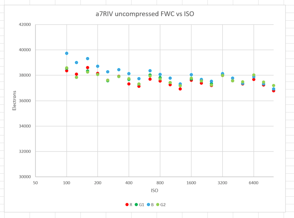
Here’s what I got for FWC:
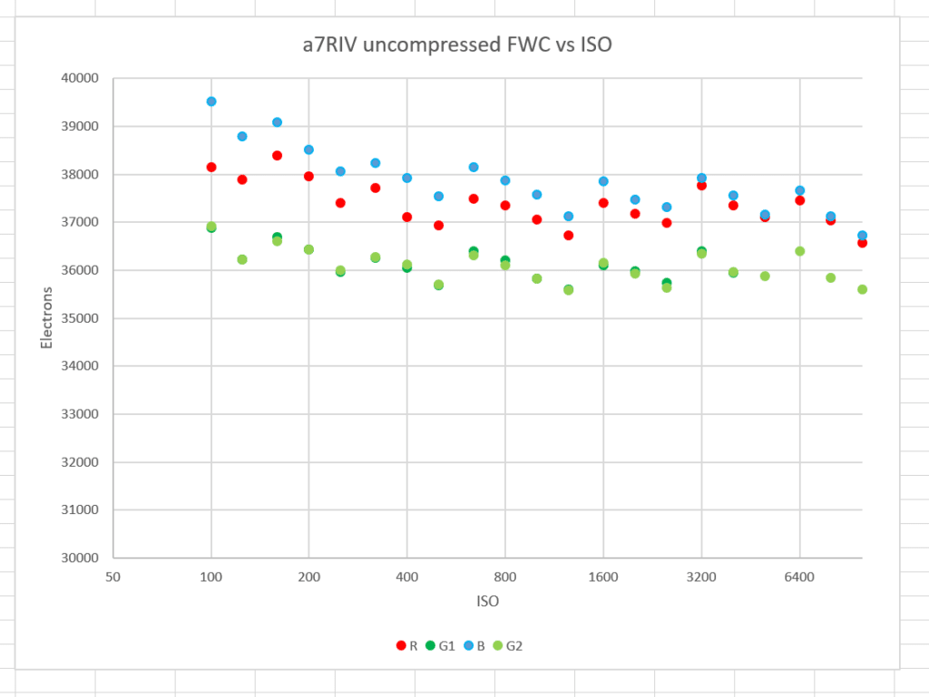
I made separate measurements on each of the raw channels at each ISO from 100 through 12800. Then I calculated the FWC at base ISO from each set. That’s what’s plotted above. The reason to do all the testing at all the different ISO settings is to catch errors and abnormalities in the camera. For example, if the capacitance ratio between the low-conversion-gain and high-conversion-gain ISO settings were wrong, there’d be a discontinuity in the scatter.
From this, I conclude that the base ISO FWC of the a7RIV is about 37000 electrons. This is lower than I measured with the GFX 100, which is a surprise. It may be that the processing the GFX 100 does to suppress PDAF banding has confused my calculations.
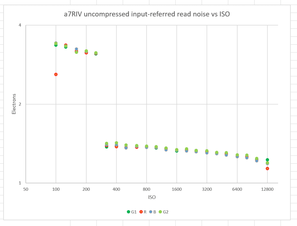
Now that we know the FWC, we can compute the read noise in terms of electrons on the photodiode:
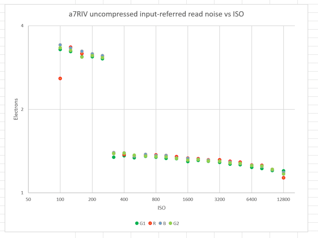
I don’t know what that red-channel outlier at ISO 100 is. I suggest ignoring it. You can see the Aptina DR-Pix algorithm doing its job in the sudden drop in read noise upon the transition from ISO 250 to ISO 320, at which point the camera switches into high-conversion-gain mode. You can also see that the camera is essentially ISOless above ISO 320.
The photon transfer curve also allows the calculation of photographic dynamic range (PDR). I’m uins Bill Claff’s definition, which is full scale divided by the mean signal level that, when referenced to an 1600-pixel-high print, gives a signal to noise ratio of 10. The plots that I now use gives more information thatn that. Let’s take a look at one:
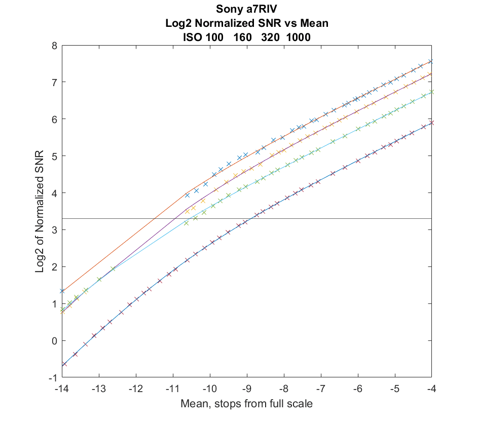
The horizontal axis is the mean signal level in stops from full scale. The rightmost part of the graph is 4 stops down from full scale, so we’re already at middle or dark gray there, and it gets darker as you go to the left. The vertical axis is the signal to noise ratio normalized to a 1600-pixel-high print. The crosses are measurements, and the lines are modeled data; they are in agreement. The black line at 3.3 marks the Claff PDR threshold (log base 2 of 10 is 3.3). The Claff PDR is measured by looking at where each curve crosses the black horizontal line. Bill gets’ 11.6 for the a7RIV PDR at base ISO. Using completely different methods, I get about the same.
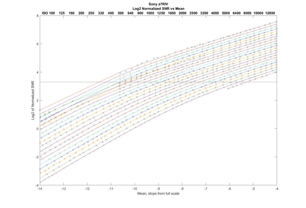
If you want to see all the ISOs, here goes:
With some advice from Jack Hogan, I’ve corrected the read noise and FWC graphs to take into account the prescaling gains that the a7RIV employs.
The FWC is a bit higher now. The RN in electrons is a bit higher, too. The shadow SNR curves look about the same.
Again, a lot of thanks for doing this!
I was suspect about Bill’s numbers since Bill’s method may get very confused: it assumes that a RAW converter would NOT compensate for the skips due to the digital gain. If the skips happen close to the black point, and the spread in the histogram is very narrow (= low ISO), this may have major results. (I think I saw his numbers off up to 0.4 steps due to this effect.)
However, your histograms show that the skips are symmetric (maybe not about “the real black”, but at least about 511 — or is it 512?), and your crosses follow closely the modeling curves… So it looks like these numbers are stable w.r.t. the strategy of the RAW converter w.r.t. the digital gain.
Did not I miss something? Do you think my argument makes sense?
Any idea why the ISO100 curve is so wiggly Jim?
No. 14 bits ought to be enough to quantize it well, considering the amount of read noise.
Jim, I do not see what the read noise can do with the curve for ISO=100. Except for 1 point (which is too far to contribute to wiggliness, being too far away), S/N ratio on this curve is ≥16. This means that the electron noise is ≥16e.
Now √(16²+4²) ≈ 16.5. The difference of 3% with 16 would not be seen on your graph.
Jack, the wiggliness must be due (as for all the similar graphs) to the digital magnification, which is the same as the gaps in histrograms. Every gap shows that the “local” contrast is (artificially) magnified 2x (here “locality” is in terms of brightness, not closeness on the sensor).
Of course, such atrocities cannot improve “the information content”, hence the noise must be affected more than the signal. So while we increase brightness, when the center of “the bell-curve histogram” passes through such a gap, this leads to decrease in S/N ratio. Or, on the graphs above, to a bump showing an increase in noise.
With the position of gaps symmetrical w.r.t. the black level (which other data from Jim confirms), the bumps should be at odd multiples of the 1st position of a gap. (The log-scale on the horizontal axis hides this, somewhat.) However, I suspect that Jim did not measure the “interesting” part, where the multiples are very small.
⁜⁜⁜⁜⁜⁜⁜⁜⁜⁜⁜⁜⁜⁜⁜⁜⁜⁜⁜⁜⁜⁜⁜⁜⁜⁜
This is why in the previous comment I said that I do not trust Bill’s numbers. Before fitting the curves, one should either “doctor” the raw data to remove the gaps (as any sensible RAW converter would do), or introduce the gaps into the mathematical model of the fitted curves. (The second alternative may be easier.)
Before this, I would not trust these curves TOO much.
The vertical axis for the curves plotted are for SNR = 10 normalized to 1600 pixels high. For the a7RIV, the normalizing divisor is 6336/1600, or about 4. SO the SNR threshold for the Claff PDR is 2.5.
Jim, your data for noise in electrons is way higher than what Bill supplies on
http://www.photonstophotos.net/Charts/RN_e.htm#Sony%20ILCE-7RM4_14
Do you have any idea why the discrepancy is so large? I do not think I saw such mismatches before…