This is one in a series of posts on the Fujifilm GFX 100S. You should be able to find all the posts about that camera in the Category List on the right sidebar, below the Articles widget. There’s a drop-down menu there that you can use to get to all the posts in this series; just look for “GFX 100S”.
A couple of days ago I tested the Fujifilm 80 mm f/1.7 G-mount lens on the GFX 100S, using a Siemens star target. I presented the results as images, and let you all judge for yourselves. Some people are good at eyeballing images and sussing out what’s going on with the lens. Some like numbers. This post is for the latter group. This is my second test using the Imatest Siemens star analysis tool. I’m still feeling my way to find out what it’s good for. There are some obvious issues with MTF normalization — see the comments to this post — but I mentally assume that the curves top out at about one.
I moved closer to the target for this test, to about 7 meters, so that the star covered about 1800 pixels in each direction. That allows the Imatest software I used to estimate modulation transfer function (MTF) for low spatial frequencies. With the exception of sharpening, the rest of the test conditions were the same as before.
- ISO 100
- Manual exposure, varying the f-stops
- Arca Swiss CA on RRS legs
- 2-second self timer
- Focusing at taking stop.
- Three images at each test condition, picked the sharpest using Imatest.
- Developed in Lr 10.2 with default settings except for white balance and sharpening.
- White balanced to the lower right gray background of the Imatest Siemens star
- Sharpening turned off.
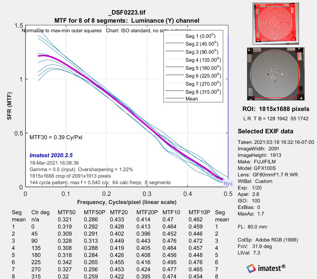
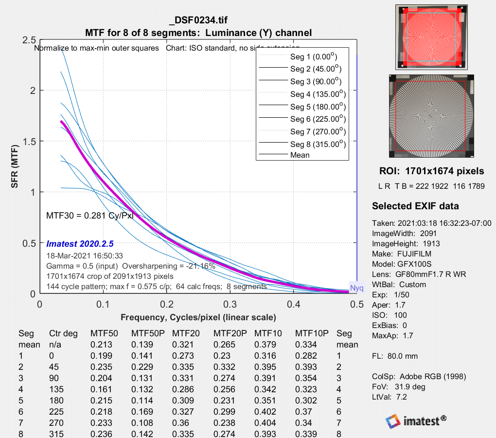
MTF in several directions in the center at f/1.7:

This is very credible performance, showing some contrast right up to the Nyquist frequency.
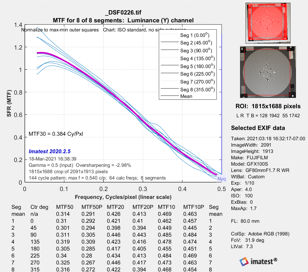
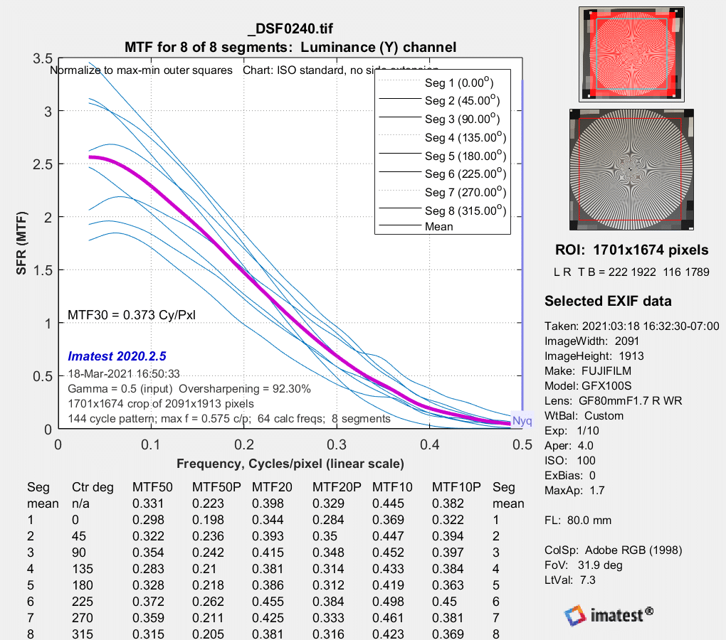
Stopping down to f/2.8:
There is modest improvement.
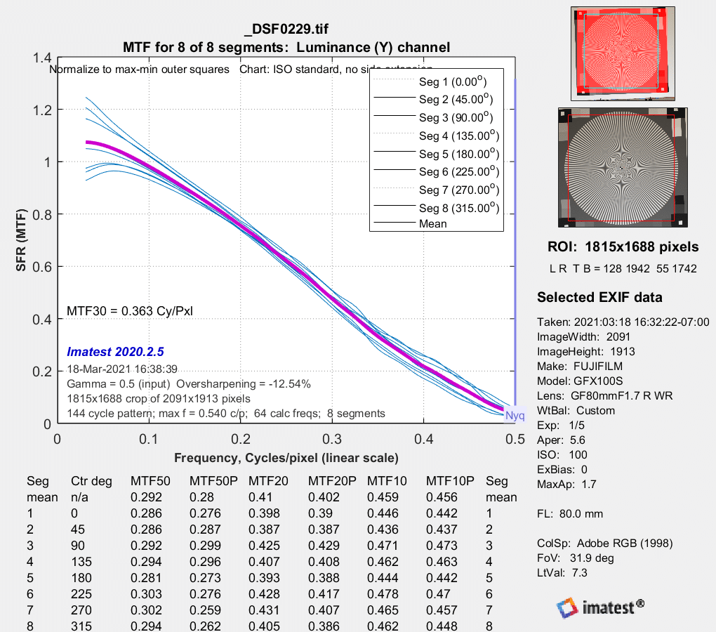
Now f/4:
About the same
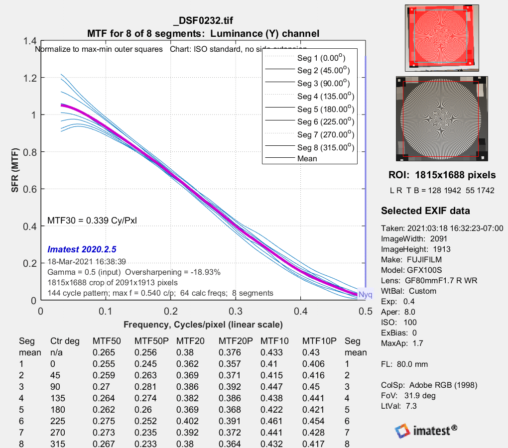
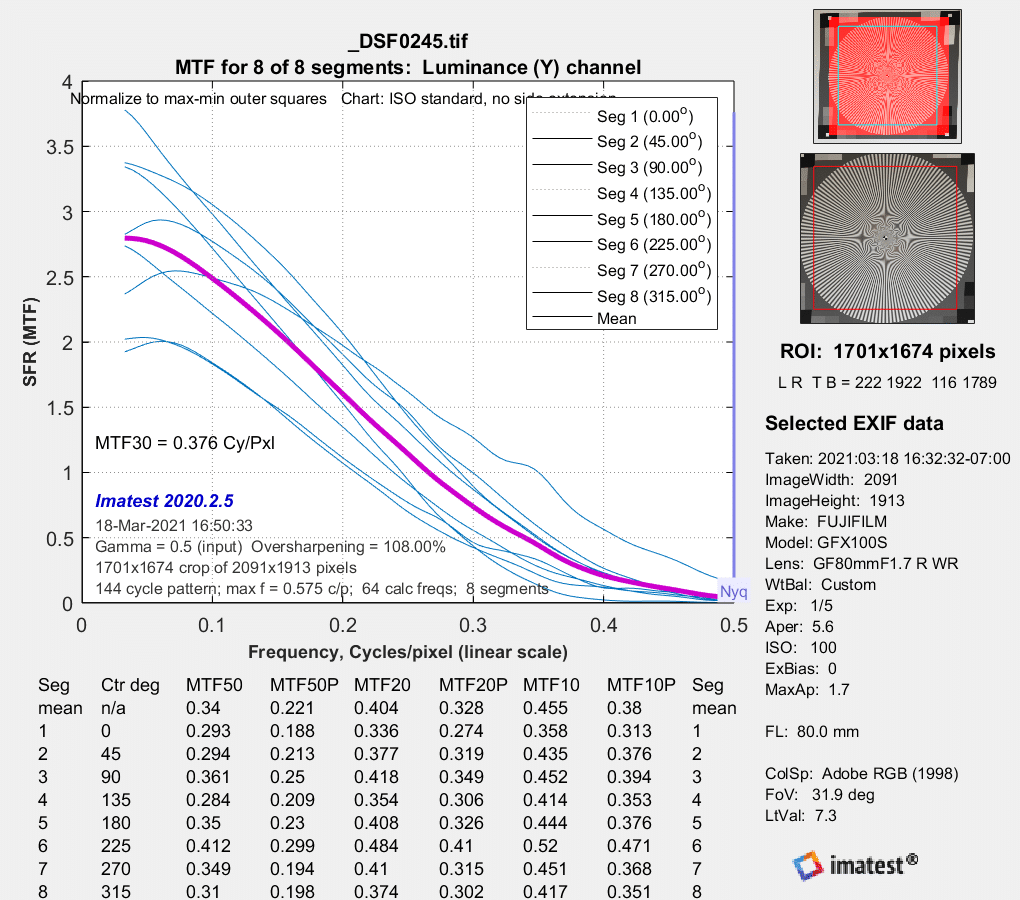
F/5.6:
A bit softer.
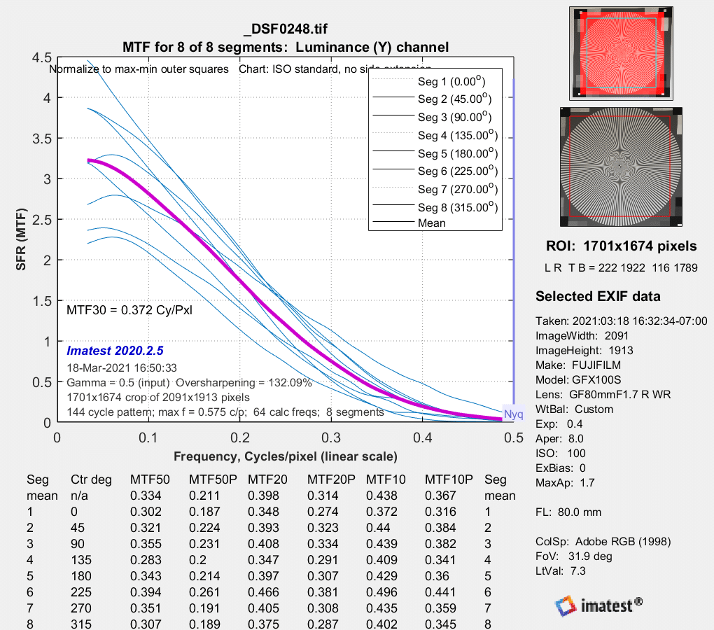
F/8:
Quite a bit softer.
That was pretty boring. How about in the upper right corner?
F/1.7:
There is a large disparity depending on the angle. I’ll provide a way to visualize what’s going on further down the page.
F/2.8:

Overall, the image is quite a bit sharper.
F/4:
Sharper yet.
F/5.6:
About the same.
F/8:
Still about the same.
The best overall f-stop looks to be f/4 or f/5.6.
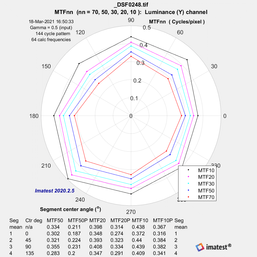
Here’s a set of charts that will make it a bit easier to see which directions are good and which are not so good.
f/1.7:
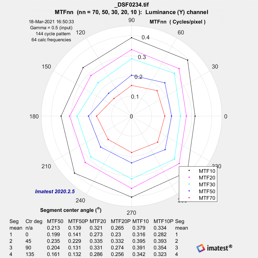
These plots need a bit of explication. Here’s what Imatest has to say about them:
The plot,…shows MTF70 through MTF10 displayed in polar coordinates. Spatial frequency (cycles per pixel in this case) increases with radius. (This is the opposite of the image itself, where spatial frequency is inversely proportional to radius.)
This plot is most similar to the spider plot shown in Image Engineering digital camera tests and Digital Camera Resolution Measurement Using Sinusoidal Siemens Stars (Fig. 15), by C. Loebich, D. Wueller, B. Klingen, and A. Jaeger, IS&T, SPIE Electronic Imaging Conference 2007. MTF10 (the black octagon on the right) corresponds to the Rayleigh diffraction limit.
The better the lens, the further towards the outside of the plot the data is. We’re looking at the upper right corner of the frame, so, thinking in terms of compass headings, the line from the center of the image to the corner is roughly SW to NE, and the lense is resolving better along that line. The line perpendicular to that is in the NW/SE direction, and the lens is resolving worse along that line.
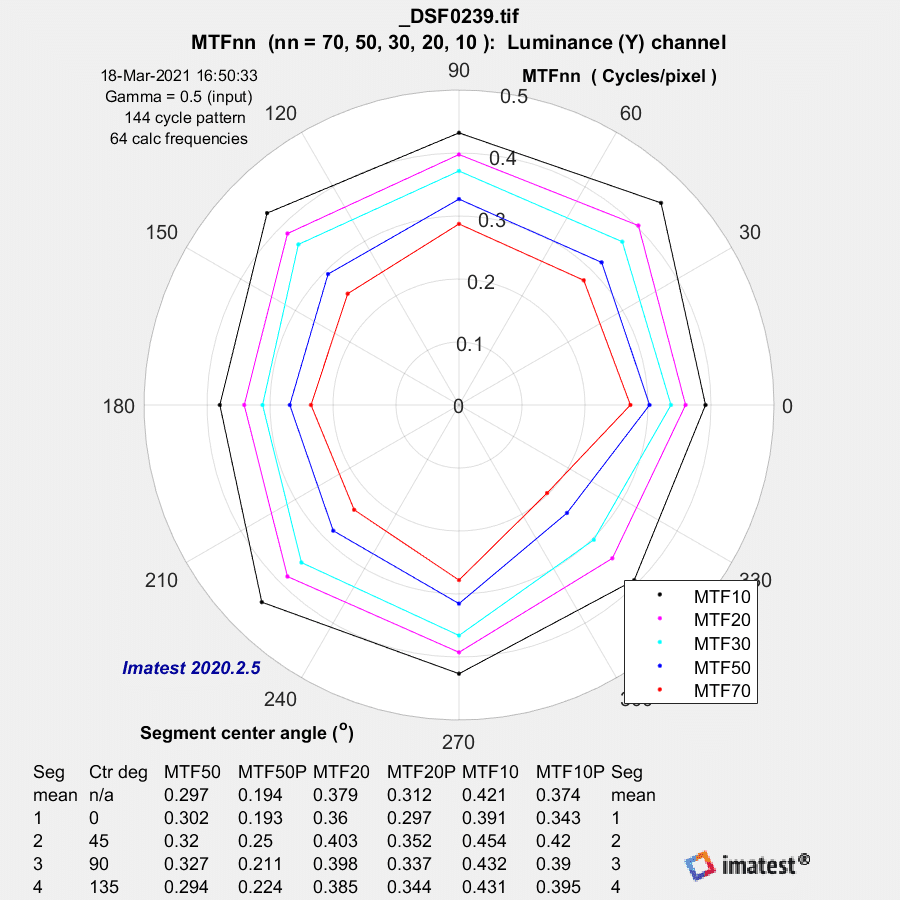
F/2.8:
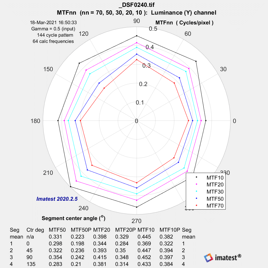
F/4:
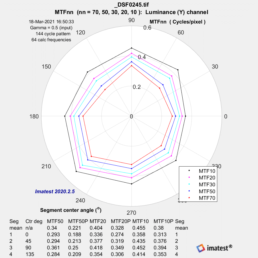
F/5.6:
F/8:
I wouldn’t place much stock in these results. I will do a more conventional slanted edge test and report on what I find.
MTF estimates approaching / running away to 3 / higher than 3. Yikes. The estimation algorithm is certainly il-conditioned, I wouldn’t trust any of it…
The normalization appears to be screwy.
Here’s what Imatest has to say on that subject:
Normalization: MTF is normalized (set to 1.0) using either (1) MTF at the outer radius of each segment, (2) the maximum value of MTF at the outer radii of all segments, or (3) the difference between the lightest and darkest square near the pattern edge. Neigher case (1) nor (2) is ideal because the minimum spatial frequency is not as low as it should be for correct normalization. (The high to low spatial frequency ratio is only 10 or 20 for the star chart — much lower than for the Log Frequency or Log F-Contrast charts.) In general, normalizing MTF to the outer radius of the star increases MTF slightly above its true value. MTF should ideally be normalized to a lower spatial frequency. Case (3) should only be used with maximum contrast patterns.
There appears to be no good answer.
Not a very satisfying explanation from them, to me. Sam Thurman wrote a nice paper on using a Siemens’ Star for MTF measurement years ago and his approach did not have these problems.
It’s not clear what they mean, either. The definition of MTF is that it is normalized by its value at the origin, which you could show is the integral over the entire PSF (understanding, there is no PSF measured here, but there are equivalent methods).
I guess if they are just getting normalization this wrong there’s a chance the shape is right, but all the measures go to zero at 0.5 cy/px. Unless the lens is atrocious, that’s not right. Visually, the lens is not atrocious, so I’d be pretty confident to say that’s not right.
I’m going to test with a conventional slanted edge.
I have no clue how to digest these plots. The center crop of Siemens star for ƒ/1.7 (one you provided a couple of days ago) shows MTF slowly descending to 0 at about 2×Nyquist frequency — as expected due to sensel sampling (then never recovering).
(In diagonal directions, it shows a zero at √2×Nyquist ¹⁾, then slightly recovering, and going again to 0 near to 2×Nyquist. So it is compatible with the description above.)
¹⁾ ???!!! I’m puzzled how this de-Bayering algorithm works — it seems to ignore non-green pixels when recoving the luminance channel?!
So it SEEMS that the slope of the MTF curve should be ½ of what the plot above shows. Do you have any comment?