• site home
  • blog home
  • galleries
  • contact
  • underwater
  • the bleeding edge

the last word

Photography meets digital computer technology. Photography wins -- most of the time.

You are here: Home / GFX 100 / Comparing the Fuji GF short primes

Comparing the Fuji GF short primes

July 8, 2021 JimK 7 Comments

This is one in a series of posts on the Fujifilm GFX 100S. You should be able to find all the posts about that camera in the Category List on the right sidebar, below the Articles widget. There’s a drop-down menu there that you can use to get to all the posts in this series; just look for “GFX 100S”. Since it’s more about the lenses than the camera, I’m also tagging it with the other Fuji GFX tags.

In the previous nine posts, I tested the off axis performance of the Fujifilm 110 mm f/2, 80 mm f/1.7 , 250 mm f/4, 63 mm f/2.8, 45 mm f/2.8, 50mm f/3.5, 30mm f/3.5, 23mm f/4, and 120 mm f/4 macro GF lenses on a GFX 100S.

In this post I’ll compare the performance of the 23, 30, 45, 50, and 63 mm primes.

Here’s the test protocol:

  • RRS carbon fiber legs
  • C1 head
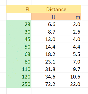
  • Target distance as per the table below
  • ISO 100
  • Electronic shutter
  • 10-second self timer
  • f/4 through f/11 in whole-stop steps
  • Exposure time set by camera in A mode
  • Focus bracketing, step size 1, 120 to 60 exposures
  • Initial focus well short of target
  • Convert RAF to DNG using Adobe DNG Converter
  • Extract raw mosaics with dcraw (I’ll change this to libraw and drop the DNG conversion when I get the chance, but the Matlab program  that controls all this is written for dcraw)
  • Extract slanted edge for each raw plane in a Matlab program the Jack Hogan originally wrote, and that I’ve been modifying for years.
  • Analyze the slanted edges and produce MTF curves using MTF Mapper (great program; thanks, Frans)
  • Fit curves to the MTF Mapper MTF50 values in Matlab
  • Correct for systematic GFX focus bracketing inconsistencies
  • Analyze and graph in Matlab
Target distance table

I analyzed a horizontal edge in the center of the frame, and both a horizontal and a vertical edge on the far right side of the frame. The horizontal edge is oriented in a radial direction, and that’s how I’m identifying it in the plots. The horizontal edge is oriented in a tangential direction, and that’s the way I’m tagging it. I also redid the tests with the target on the lens axis.  I looked at both horizontal and vertical edges. The edges are identified on the graphs as, respectively,  radial and tangential edges. Those terms don’t make sensor on axis. The numbers ought to be the same, but I’ve included both to give you an idea of the variation possible with my test method.

Here are the MTF50 results in cycles per picture height:

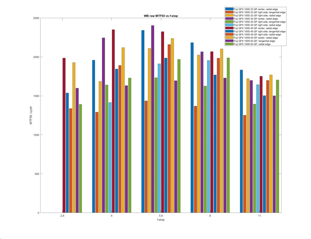
I measured the MTF50 on each of the raw channels, and am reporting on the MTF50 on a white-balanced composite of those channels, which is mostly the green channel. Unsurprisingly, the 23 struggles the most off axis. Surprisingly, that only occurs in one direction. The consistency among this group of lenses is remarkable.

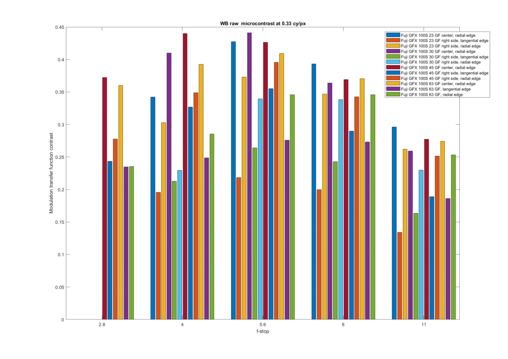
Next is the microcontrast at the tough standard of 0.33 cycles per pixel.

Now for the longitudinal chromatic aberration (LoCA).

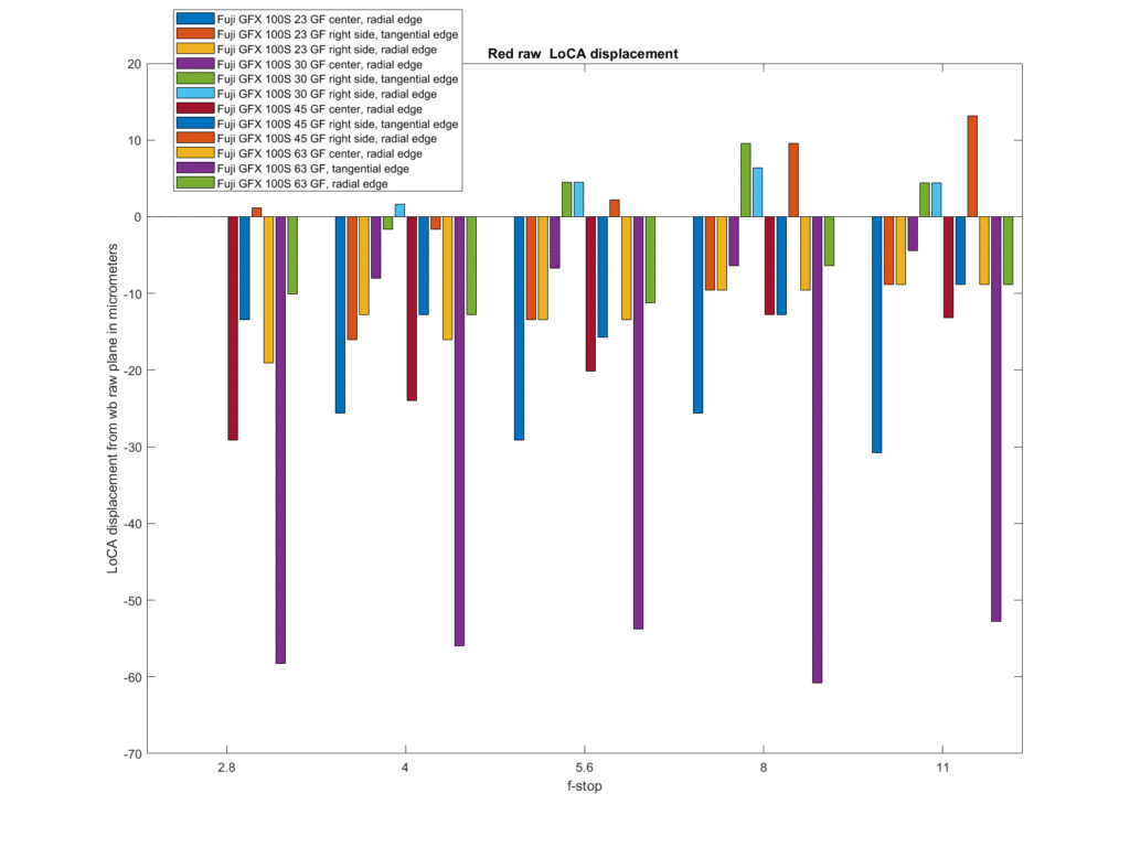
The above plots the shift of the red raw image plane (on the sensor side of the lens) compared to the white-balanced raw plane.

The GF 63 has a lot of LoCA on the right side with a tangential edge. Next worst is the 23 in the center, and that’s not bad in absolute terms.The lother look fairly low.

GFX 100, GFX 100S, GFX 50S

← Off-axis testing of the Fuji 23/4 GF on the GFX 100S Comparing the Fuji GF long primes →

Comments

  1. CarVac says

    July 9, 2021 at 8:58 am

    Perhaps line plots would be better than bar charts?

    Reply
    • JimK says

      July 9, 2021 at 9:09 am

      One line for each lens, edge orientation, and ROI position, that line plotted across all f-stops?

      Reply
  2. Scott Pilla says

    July 9, 2021 at 9:21 am

    The data display makes it tough to compare with so many lenses — keep having to look back and forth to the legend. My suggestion — make one color per lens with different luminance — like gf23 center dark red, tangential edge medium red, radial edge light red. keep that consistent across all charts.

    Reply
    • JimK says

      July 9, 2021 at 9:26 am

      And keep the plots bar charts?

      Reply
      • scott says

        July 9, 2021 at 12:29 pm

        yeah i prefer them as bar charts

        Reply
  3. Tony A says

    July 10, 2021 at 12:48 pm

    I’ll cast a vote for retaining them as bar charts, but with gaps inserted between each set. That way I could immediately distinguish one lens from another without having to refer more than once to the legend.

    Reply
  4. Tony A says

    July 10, 2021 at 12:50 pm

    Clarification: “… gaps inserted between each triad”

    Reply

Leave a Reply Cancel reply

Your email address will not be published. Required fields are marked *

May 2025
S M T W T F S
 123
45678910
11121314151617
18192021222324
25262728293031
« Apr    

Articles

  • About
    • Patents and papers about color
    • Who am I?
  • How to…
    • Backing up photographic images
    • How to change email providers
    • How to shoot slanted edge images for me
  • Lens screening testing
    • Equipment and Software
    • Examples
      • Bad and OK 200-600 at 600
      • Excellent 180-400 zoom
      • Fair 14-30mm zoom
      • Good 100-200 mm MF zoom
      • Good 100-400 zoom
      • Good 100mm lens on P1 P45+
      • Good 120mm MF lens
      • Good 18mm FF lens
      • Good 24-105 mm FF lens
      • Good 24-70 FF zoom
      • Good 35 mm FF lens
      • Good 35-70 MF lens
      • Good 60 mm lens on IQ3-100
      • Good 63 mm MF lens
      • Good 65 mm FF lens
      • Good 85 mm FF lens
      • Good and bad 25mm FF lenses
      • Good zoom at 24 mm
      • Marginal 18mm lens
      • Marginal 35mm FF lens
      • Mildly problematic 55 mm FF lens
      • OK 16-35mm zoom
      • OK 60mm lens on P1 P45+
      • OK Sony 600mm f/4
      • Pretty good 16-35 FF zoom
      • Pretty good 90mm FF lens
      • Problematic 400 mm FF lens
      • Tilted 20 mm f/1.8 FF lens
      • Tilted 30 mm MF lens
      • Tilted 50 mm FF lens
      • Two 15mm FF lenses
    • Found a problem – now what?
    • Goals for this test
    • Minimum target distances
      • MFT
      • APS-C
      • Full frame
      • Small medium format
    • Printable Siemens Star targets
    • Target size on sensor
      • MFT
      • APS-C
      • Full frame
      • Small medium format
    • Test instructions — postproduction
    • Test instructions — reading the images
    • Test instructions – capture
    • Theory of the test
    • What’s wrong with conventional lens screening?
  • Previsualization heresy
  • Privacy Policy
  • Recommended photographic web sites
  • Using in-camera histograms for ETTR
    • Acknowledgments
    • Why ETTR?
    • Normal in-camera histograms
    • Image processing for in-camera histograms
    • Making the in-camera histogram closely represent the raw histogram
    • Shortcuts to UniWB
    • Preparing for monitor-based UniWB
    • A one-step UniWB procedure
    • The math behind the one-step method
    • Iteration using Newton’s Method

Category List

Recent Comments

  • JimK on Goldilocks and the three flashes
  • DC Wedding Photographer on Goldilocks and the three flashes
  • Wedding Photographer in DC on The 16-Bit Fallacy: Why More Isn’t Always Better in Medium Format Cameras
  • JimK on Fujifilm GFX 100S II precision
  • Renjie Zhu on Fujifilm GFX 100S II precision
  • JimK on Fuji 20-35/4 landscape field curvature at 23mm vs 23/4 GF
  • Ivo de Man on Fuji 20-35/4 landscape field curvature at 23mm vs 23/4 GF
  • JimK on Fuji 20-35/4 landscape field curvature at 23mm vs 23/4 GF
  • JimK on Fuji 20-35/4 landscape field curvature at 23mm vs 23/4 GF
  • Ivo de Man on Fuji 20-35/4 landscape field curvature at 23mm vs 23/4 GF

Archives

Copyright © 2025 · Daily Dish Pro On Genesis Framework · WordPress · Log in

Unless otherwise noted, all images copyright Jim Kasson.