Off-axis testing of the Fuji 63/2.8 GF on the GFX 100S

This is one in a series of posts on the Fujifilm GFX 100S. You should be able to find all the posts about that camera in the Category List on the right sidebar, below the Articles widget. There’s a drop-down menu there that you can use to get to all the posts in this series; just look for “GFX 100S”. Since it’s more about the lenses than the camera, I’m also tagging it with the other Fuji GFX tags.

In the previous four posts, I tested the off axis performance of the Fujifilm 110 mm f/2, 80 mm f/1.7 , 250 mm f/4, and 120 mm f/4 macro GF lenses on a GFX 100S. Now I’ll do the same with the 63 mm f/2.8 lens.

Here’s the test protocol:

• RRS carbon fiber legs
• C1 head
• Target distance 5.5 meters for a 63 mm lens
• ISO 100
• Electronic shutter
• 10-second self timer
• f/2.8 through f/11 in whole-stop steps
• Exposure time set by camera in A mode
• Focus bracketing, step size 1, 120 to 60 exposures
• Initial focus well short of target
• Convert RAF to DNG using Adobe DNG Converter
• Extract raw mosaics with dcraw (I’ll change this to libraw and drop the DNG conversion when I get the chance, but the Matlab program  that controls all this is written for dcraw)
• Extract slanted edge for each raw plane in a Matlab program the Jack Hogan originally wrote, and that I’ve been modifying for years.
• Analyze the slanted edges and produce MTF curves using MTF Mapper (great program; thanks, Frans)
• Fit curves to the MTF Mapper MTF50 values in Matlab
• Correct for systematic GFX focus bracketing inconsistencies
• Analyze and graph in Matlab

I analyzed a horizontal edge in the center of the frame, and both a horizontal and a vertical edge on the far right side of the frame. The horizontal edge is oriented in a radial direction, and that’s how I’m identifying it in the plots. The horizontal edge is oriented in a tangential direction, and that’s the way I’m tagging it. Because I was suspicious of some of the numbers that I’d gotten for the 63 in the past, I also redid the tests with the target on the lens axis.  I looked at both horizontal and vertical edges. The edges are identified on the graphs as, respectively,  radial and tangential edges. Those terms don’t make sensor on axis. The numbers ought to be the same.

Here are the MTF50 results, in cycles per picture height:

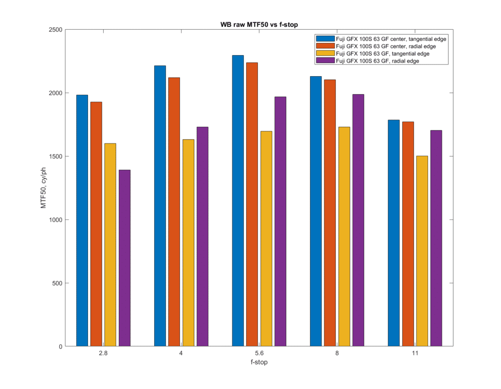
I measured the MTF50 on each of the raw channels, and am reporting on the MTF50 on a white-balanced composite of those channels, which is mostly the green channel. I got much better performance from the 63 on-axis at f/2.8 and f/4 than I did before.

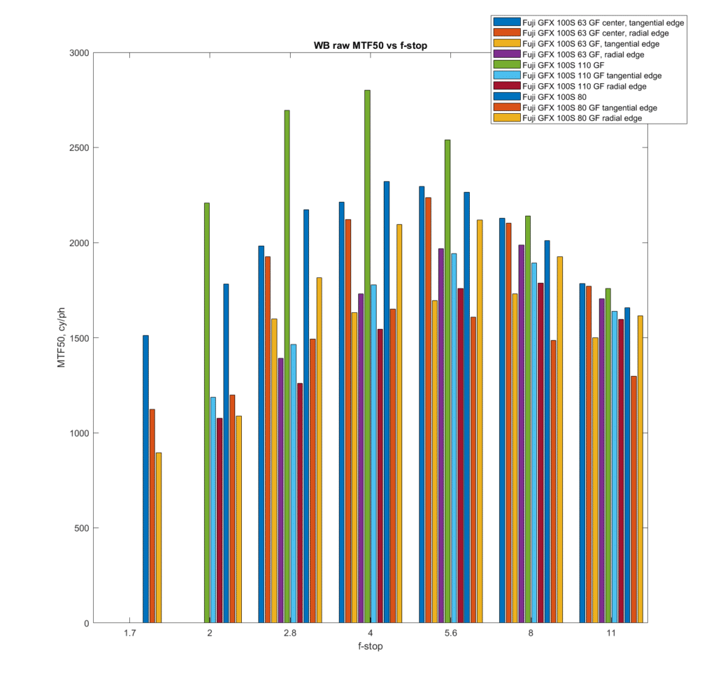
To put that in perspective, here is an MTF curve with the 110/2 and 80/1.78 added:

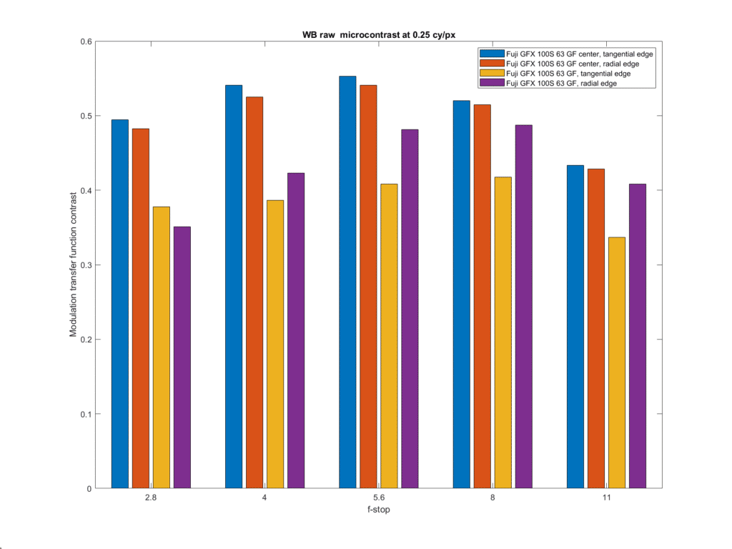
Another way to look at sharpness is microcontrast, which is defined as the contrast at a particular frequency not far from Nyquist. I prefer 0.25 cycles per pixel.

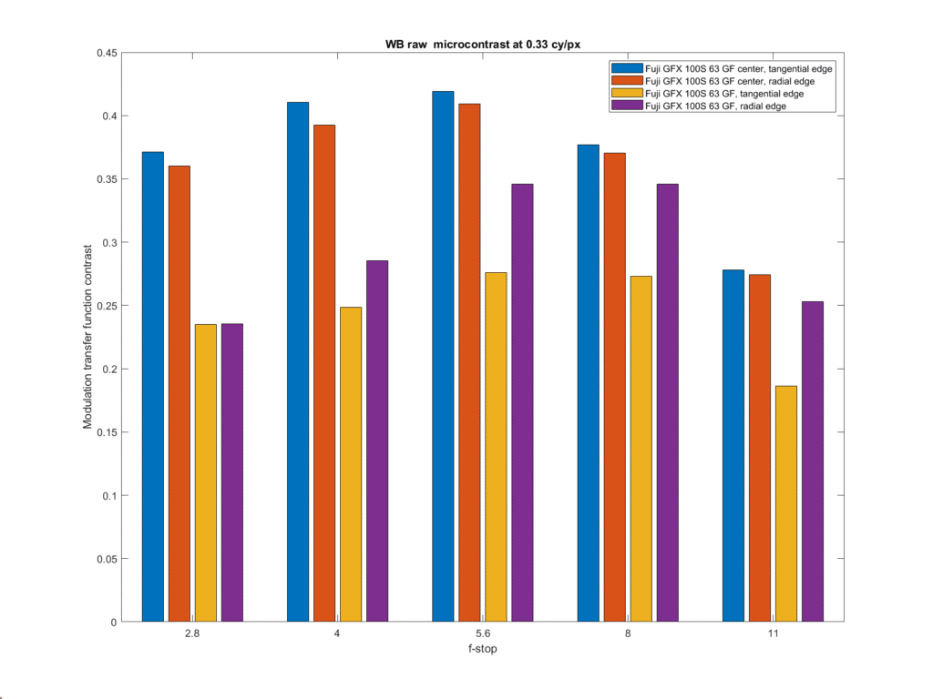
Tightening the standard to 0.33 cycles per pixel:

Next is longitudinal chromatic aberration (LoCA) by the numbers; I’ll include the 80 and 110 for comparison.

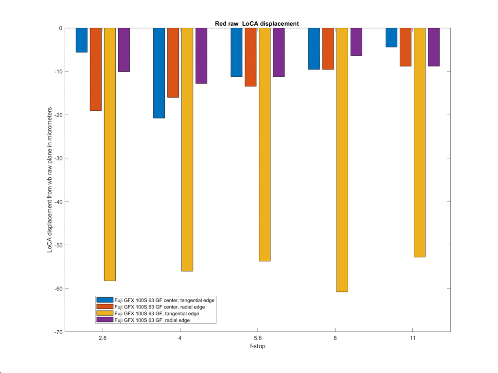
This plots the shift of the red raw image plane (on the sensor side of the lens) compared to the white-balanced raw plane. LoCA is pretty low except for the tangential edge on the side of the image.

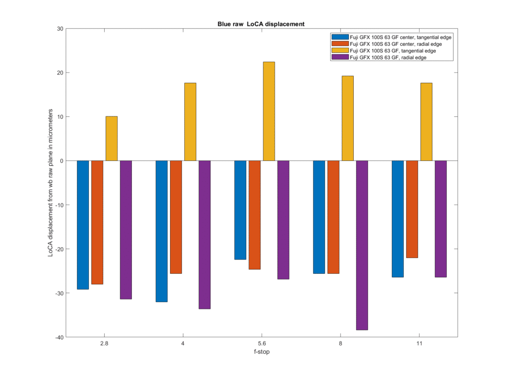
The tangential edge at the side of the image is also an outlier for blue LoCA.

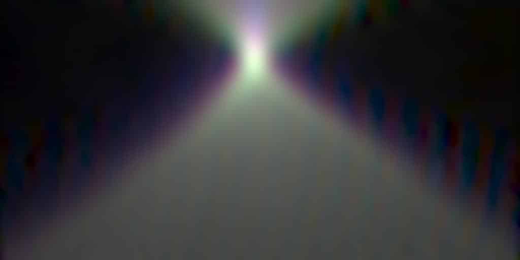
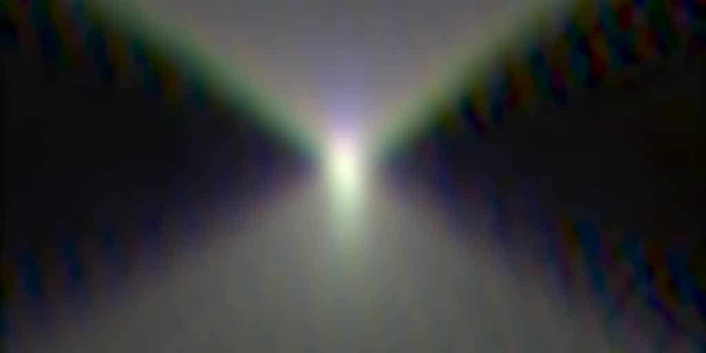
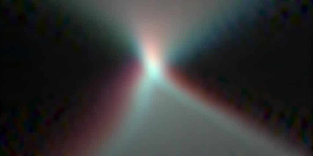
There’s another way of looking at LoCA and defocusing behavior, and that’s what I’m calling the transfocal bokeh images.

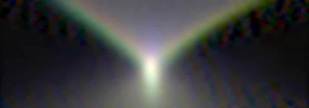
The vertical direction is the shift of the focal plane with respect to the plane of the sensor. Focus distance runs from top to bottom, with front-focused at the top and back-focused at the bottom. The horizontal axis a heavily-magnified view of distance in the sensor plane. The colors are highly approximate; I just assigned the raw channels to their respective sRGB channels.