Warning: this is a technical post that assumes a fair amount of knowledge on the part of the reader.
Jack Hogan and I have been working on photon transfer analysis of sensors for some time. He and I wrote some Matlab code to analyze pixel response non-uniformity (PRNU), to plot complete photon response curves, and to model sensor behavior. At present, the suite of programs does not analyze dark frame-to-frame persistent patterning, although I have done some of that in the past.
For all the testing except the PRNU, captures are made in pairs. By subtracting a pair of images, a image with 1.414 times the frame-independent noise, unpolluted by static noise, can be obtained, Earlier work did the captures of flat fields; one pair of images was needed for each point of the photon transfer curve (PTC). A PTC plots standard deviation versus mean value, usually using a log scale for both. While using a pair for every data point promoted accuracy, it was truly labor intensive; one set of exposures for each ISO setting for a given camera could number in the mid- thousands.
In order to reduce the number of necessary captures, I created first a one-dimensional, and then a two-dimensional target. Here is the one that I’m currently using:

I made it in Photoshop, and it’s far from perfectly linear in density from side to side and top to bottom, nor does in optimally minimize duplicated tones. I could create a better target using Matlab, and I probably will, but, as you will soon see, this one is adequate for the purpose I have in mind.
You will note the absence of patches in the target. The patches are created by the software sampling the target, and they can be any convenient shape, size, and number. The fact that the target is a gradient is not important for any single patch, since subtracting the two samples takes that out of the picture. It is important to keep the sample extents small enough that most of the sampled values are close together. That must be balanced against wanting many pixels in each sample for the purpose of having solid statistics. As it turns out, with today’s high-resolution cameras, that is no problem.
The capture protocol that I have selected is to make a set of pairs at each camera ISO setting of interest using aperture priority, exposure compensation to get the upper left corner near full scale, and varying the ISO setting. That gets the upper end of the photon transfer curves for each ISO.
I also need a set of exposures nearer, but not at, the black point, which I can use to model the read noise of the camera. To get rid of quantizing artifacts, I have the program throw away samples with SNRs of less than 2, so very dark values are automatically eliminated. If the camera under test were completely ISOless, the same exposure would suffice for each dark capture, no matter what the ISO setting. My hope was that the target would have enough dynamic range so that one exposure setting would suffice even in cameras that significantly depart fro ISOless behavior. So far that has worked out.
What should the exposure be for the dark images. I hoped to get five or six stops of sample variation per exposure, so that the first set of captures would span a range from half a stop or a stop under full scale to fice or six stops below that. Modern cameras have engineering dynamic ranges of about 14 stops. I don’t need to get that far down on the curve, since I”m going to toss the samples with an SNR of less than 2, but I do want to get to 13 or so stops down. Setting the exposure for the dark series at 7 stops less than the base ISO exposure for the light series should get me there.
Enough theory. What happens in practice?
Here are measured and modeled photon transfer curves for the Sony a7RII at whole stop ISOs from 100 to 12800, using a 4×6 grid of equally spaced 400×400 pixel samples.
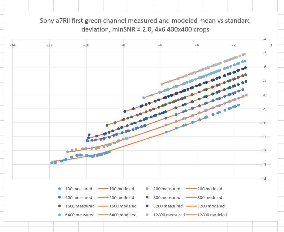
The blue dots are the measured values, the orange lines are the modeled ones. The horizontal axis is the mean sample value. The vertical axis is the standard deviation. You can see by looking at the right hand side of the graph at the three lower curves, that the target dynamic range is less than the six stops that I’d like. What if we have 48 300×300 pixel samples instead or more bigger ones?
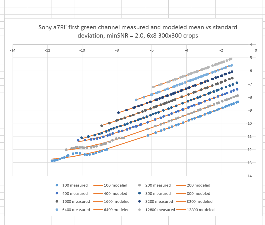
That’s better. Almost six stops. There’s no longer a gap in the ISO 400 measured curve. If a little increase in sampling density is good, is a lot better? Let’s look at 96 200×200 pixel samples.
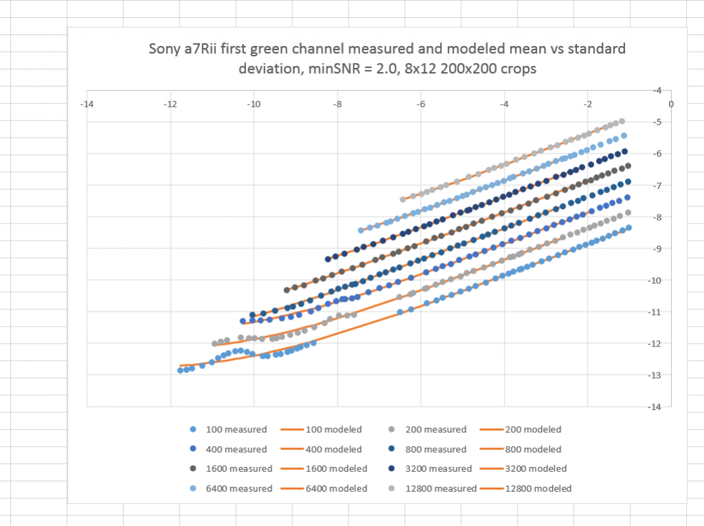
Better yet. I think I’ll stop there, though.
Now notice the gaps in the ISO 100 and ISO 200 curves. That’s because we didn’t sample the lower middle of their dynamic range. That’s not a problem, though. The middle of the dynamic range is almost always completely boring. It’s the most linear region. It doesn’t affect the modeling much at all. No great loss; in fact, no piratical loss at all.
And the waviness to the ISO 100 and the ISO 200 measured values? We’ve seen that before on other cameras that have read noise comparable to their quantizing LSB. I had the camera set to compressed raw, so the a7RII was acting as a 13 bit camera.
Success. The capture time for the PTC data is now a few minutes, and all I need is a 100 or so images.
Leave a Reply