In this article, there is the following statement:
How precise are tables and depth of field calculators?
Usually most tables pretend to have a precision that is neither available nor sensible in reality. That is partly because the values calculated in the tables are based on the arbitrary specification of a limit value (acceptable circle of confusion diameter).
In reality, however, the sharpness is continuously changing in the depth and its subjective perception is also somewhat based on the image content in addition to the viewing conditions. There is therefore no clear limit!
The from-to tables with millimetre precision at meter distances, on the other hand, easily give the impression that there are two precisely positioned flat limit surfaces in front of the camera between which everything is displayed at constant sharpness. But there are a few things wrong with this notion.
Most tables and calculation programs found on the internet are based on the geometric model of the light cones and circles of confusion that we have also been using for illustration. Yet despite how nice it is, it is only an idealization of the real optical processes in a lens. That is because this model does not recognize aberrations, colours, or diffraction. In the geometric model, the circle of confusion is a disc with even brightness.
In reality, however, the distribution of brightness in the focused and lightly unfocused point image is uneven. We will deal with that in more detail below. All types of aberrations from real lenses cause a series of deviations from the geometric model:
• In ideal lenses, the image-side depth of focus grows nearer and farther away at the same rate when the aperture is made narrower. In real lenses, however, there can be a displacement to one side called the focus shift. When it is very large, the near limit of the depth of field range might remain unchanged when the aperture is narrowed.
• Away from the optical axis, this shift often has opposite direction compared to the centre of the image, the depth of field space is then curved.
• If lenses suffer form vignetting by parts of the lens barrel, then the depth of field at the edge of the frame is larger than in the centre because the size of the pupil decreases due to the vignetting.
• Depending on the lens aberration, the type of blurriness can be different in front of and behind the focal plane.
• The location of the depth of field range also depends somewhat on the colour of the light.
The usual tables and calculators therefore provide some useful clues for practice, but they should not be taken too seriously.
All of that is true, and I’ve reported on much of that many times in this blog. But the quoted material, especially the last sentence, can be taken to mean that DOF calculations and DOF calculators are not generally useful. Are they?
I think they are, in many contexts. In this post I’ll examine the usefulness of those calculators in the context of landscape photography using one example.
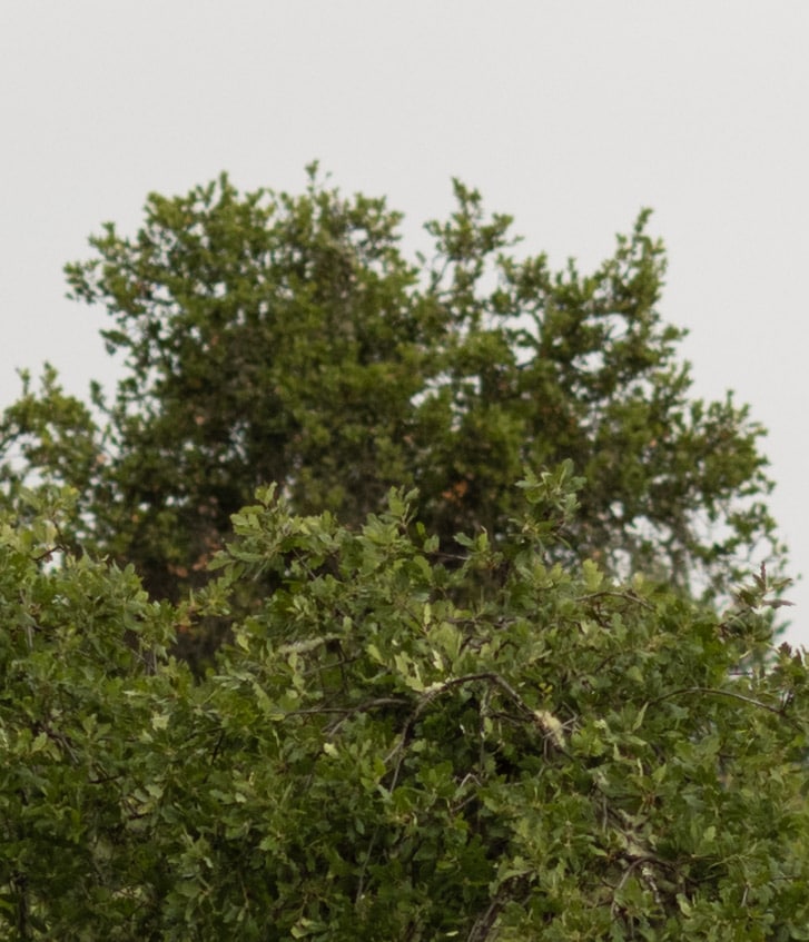
The example I’m going to show you is a series of images of this scene:
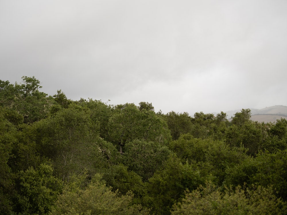
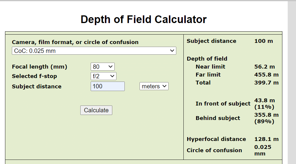
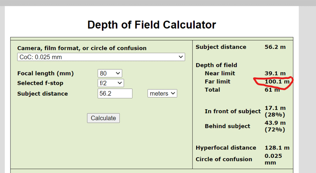
The tree against the sky in the middle of the image is 101 meters from the camera, and the tree immediately in front of it is 55 meters away. I have shown you crops at various f-stops that show how much the “foreground” tree is blurred, and what the circle of confusion diameters (CoCs) are at those stops when geometric optics, which is what’s behind DOF calculators) is used to calculate the DOF.
The 80 mm f/1.7 GF lens I used on the GFX 100S for these shots is not particularly well-corrected; in particular, it suffers (or benefits, depending on your point of view) from analmolous transfocal behavior. Therefore, especially at the wider apertures, if there are departures in blur from what the DOF calculators predict, we ought to see it with this lens. What I am doing to test that is to compare actual images of the foreground — 55 meter — tree when the camera is focused on the background — 100 meter — tree, with sharp images of the foreground tree that have been blurred in precisely the way that geometric optics assumes. So we’re going to compare the foreground tree using an actual lens with the foreground tree that the DOF calculators think the lens is producing.
Where did I get the image with the foreground tree sharp? I made a shot at f/4 after focusing on the foreground tree.
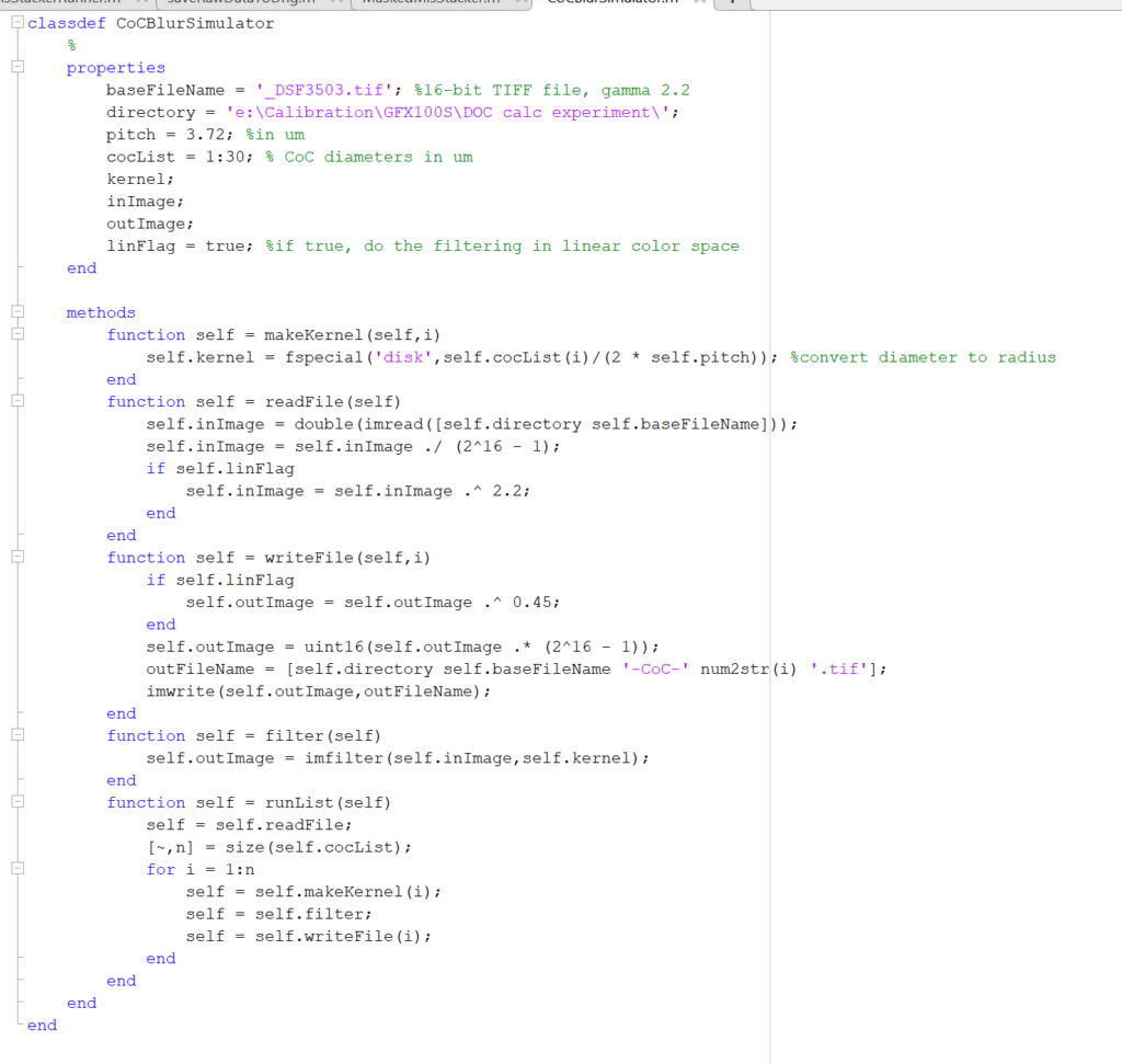
I used some Matlab code to apply the pillbox filters to the images. If anybody is interested, here it is:
With an f-stop of f/2 for the real image, and the simulated CoC of 23 um for the simulated one at 100% magnification:
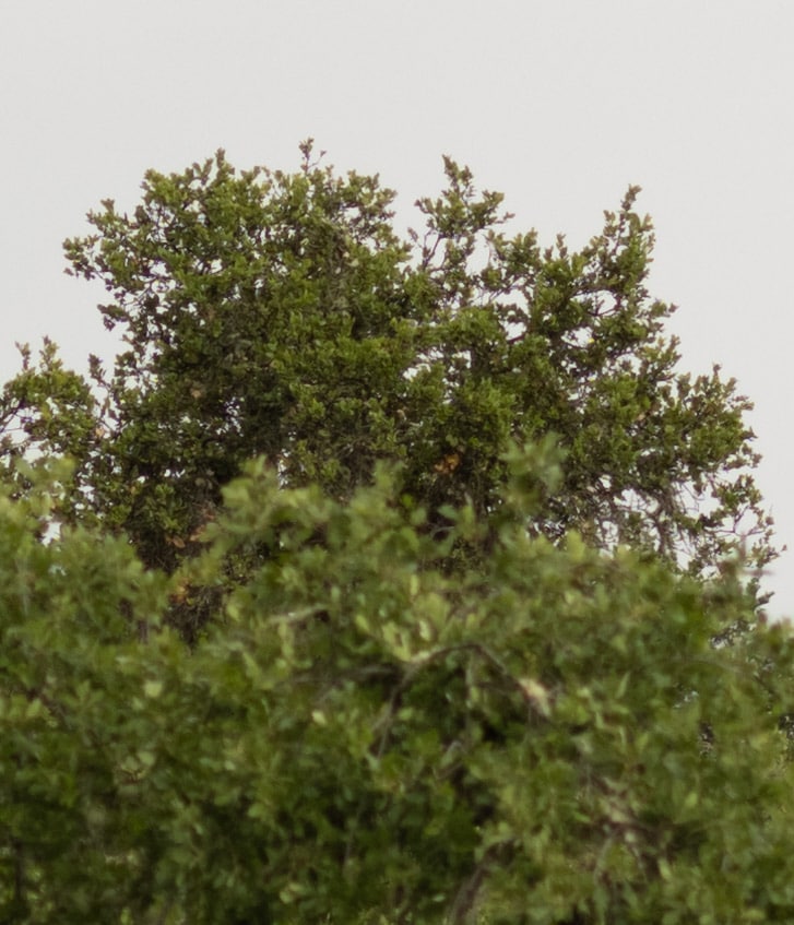
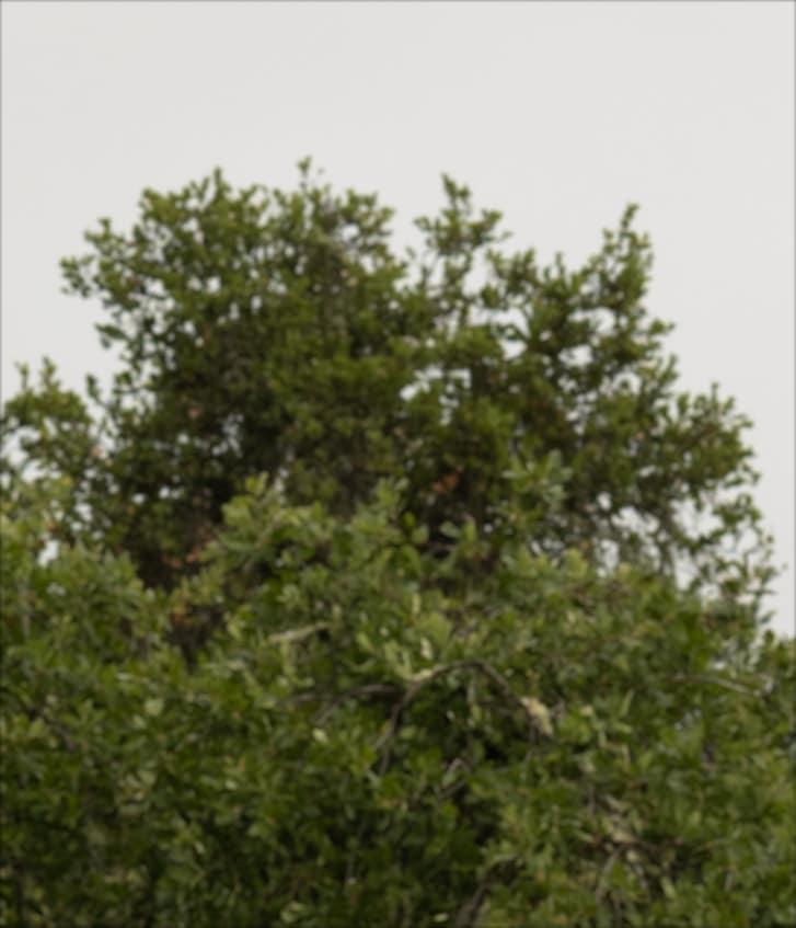
Geometric optics states that the CoC of the foreground tree should be 25 um, but that gives just a tad more blur than the unmanipulated image. So, in this case, the actual lens has a bit more DOF than geometric optics says it should have.
The Zeiss paper talks about asymmetrical DOF, which does indeed exist.
Geometric optics assumes that doesn’t happen:
If we focus on the front tree and look at the back tree, we should see the same amount of blur that we see if we focus on the back tree and look at the front tree.
Do we?
To me, the back tree looks a bit sharper when we focus on the front tree than the front tree looks when we focus on the back tree.
Let’s take an f/4 image focused on the back tree and apply the blur implied by the CoC that we get from geometric optics and see what that looks like.

That’s a bit blurry; 21 um is a better match.

So we do observe a slight asymmetry, and also that the actual lens has somewhat more DOF than what we compute from geometric optics.
I can, and probably will, explore other apertures with this lens, but in this case, I think the DOF calculators are quite a useful approximation to what we actually see with the 80/1.7 GF at f/2.
Field curvature, as pointed out in the Zeiss paper, can be a confounding issue. In the case of lenses with significant field curvature, I prefer to think of DOF as departures from the surface of sharp focus, rather than the plane of sharp focus. Focus shift is another issue, and in the case of the GFX cameras, can be easily dealt with by focusing at the taking aperture, or at least the aperture narrower than which focus shift is no longer an issue.
Leave a Reply