This is the second post on balancing real and fake detail in digital images. The series starts here.
In the last post I looked at the amount of aliased and correctly reconstructed image detail in the case of a monochromatic sensor an ideal lens, in combination with some spherical aberration and defocusing. The calculations assumed an ideal point sampler. Since real camera sensors are far from point samplers, it makes sense to look at the reduction in aliased detail that occurs if you assume a more realistic sensor model.
The model I chose is a uniform square, the length of whose sides is the pixel pitch times the square root of the fill factor. Thus, for a fill factor of 100%, the whole receptive area is equally receptive, and the length of the sides is equal to the pixel pitch. For a fill factor of 50%, the length of the sides of the receptive area is 0.707 times the pixel pitch. There is a fairly simple analytic solution if the receptive area is a circle or if it is circularly symmetric, but I thought that was too far from reality, so I used numerical methods that I learned from Jack Hogan’s great blog, Strolls with my Dog. It is possible to lower execution times by employing hybrid — part analytical, part numerical — methods; trying to keep the programming simple, I didn’t do that for the results reported here.
Because the receptive area of the modeled pixel is not circularly symmetric, MTF will vary with direction. I am reporting on the MTF in the vertical and horizontal direction. The MTF measured diagonally will be higher.
Here’s the difference in MTF’s for a point sampler (the red lines) and a sensor with a fill factor of 100%:

The horizontal axis is in cycles per millimeter. It’s easier to tell where aliasing occurs if we convert that to cycles per pixel:
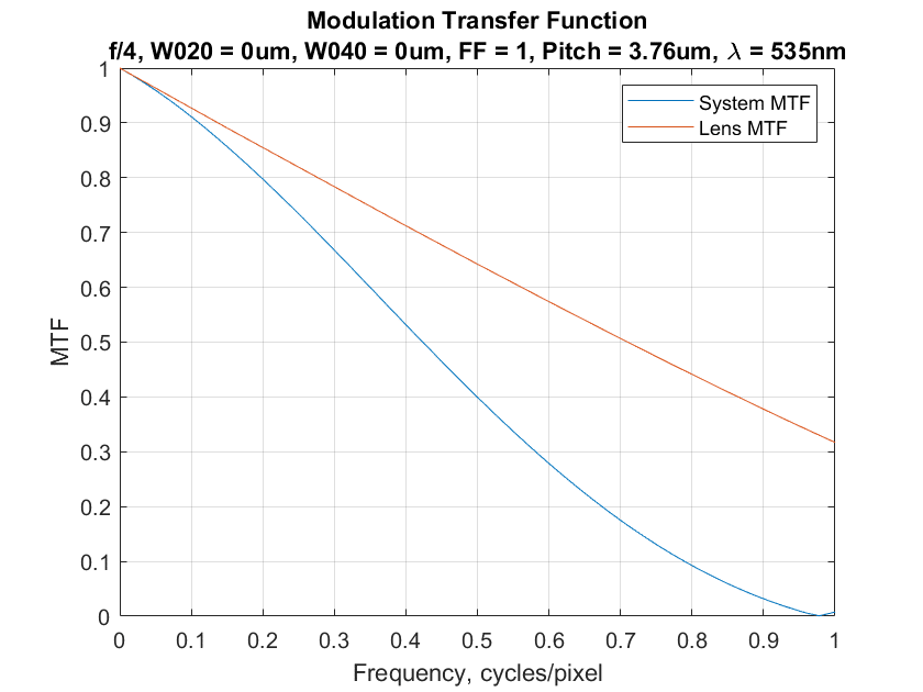
The Nyquist frequency is 0.5 cycles per pixel, so MTF’s greater than zero to the right of that mean aliasing is possible, and, if the subject has sufficient high-spatial-frequency contrast, inevitable.
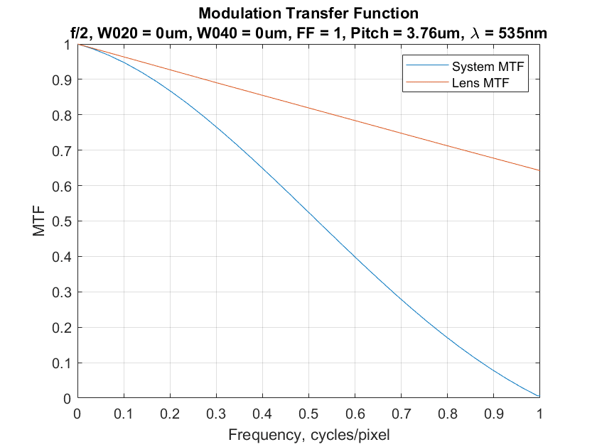
At wider f-stops, the 100% fill factor helps reducing aliasing even more:
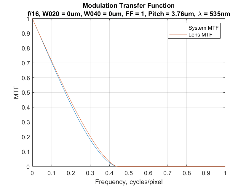
And at narrower f-stops, it helps less:
Here’s what the curves look like across a range of f-stops:
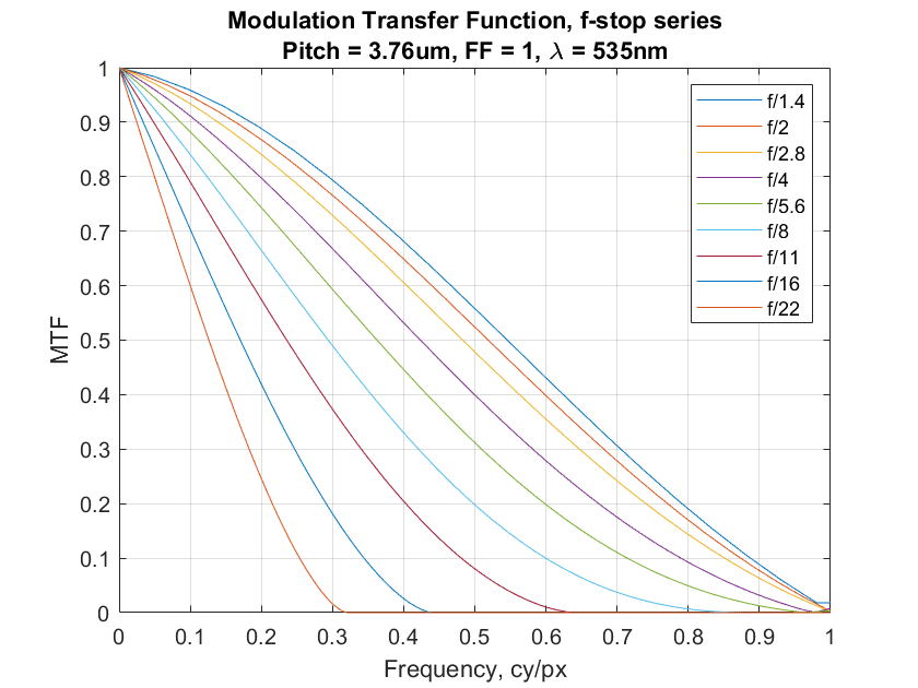
The f/1.4 curve is approaching the curve of a system with a diffractionless lens.
In the last post, I presented a metric for the amount of real and aliased detail that can be recorded: the average MTF below and above the Nyquist frequency. The former is a measure for real detail, and the latter a measure of falsely reconstructed scene data.
Here’s how those two metrics vary over a range of f-stops:
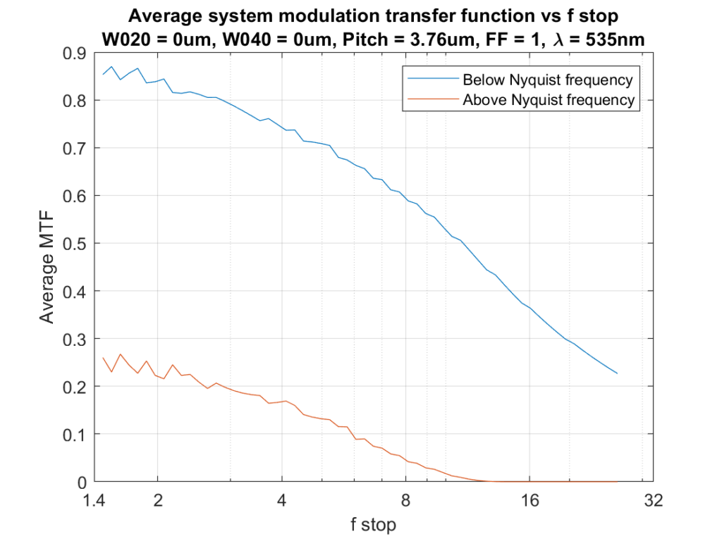
That looks quite a bit better than the same set of curves for a point sampling sensor.
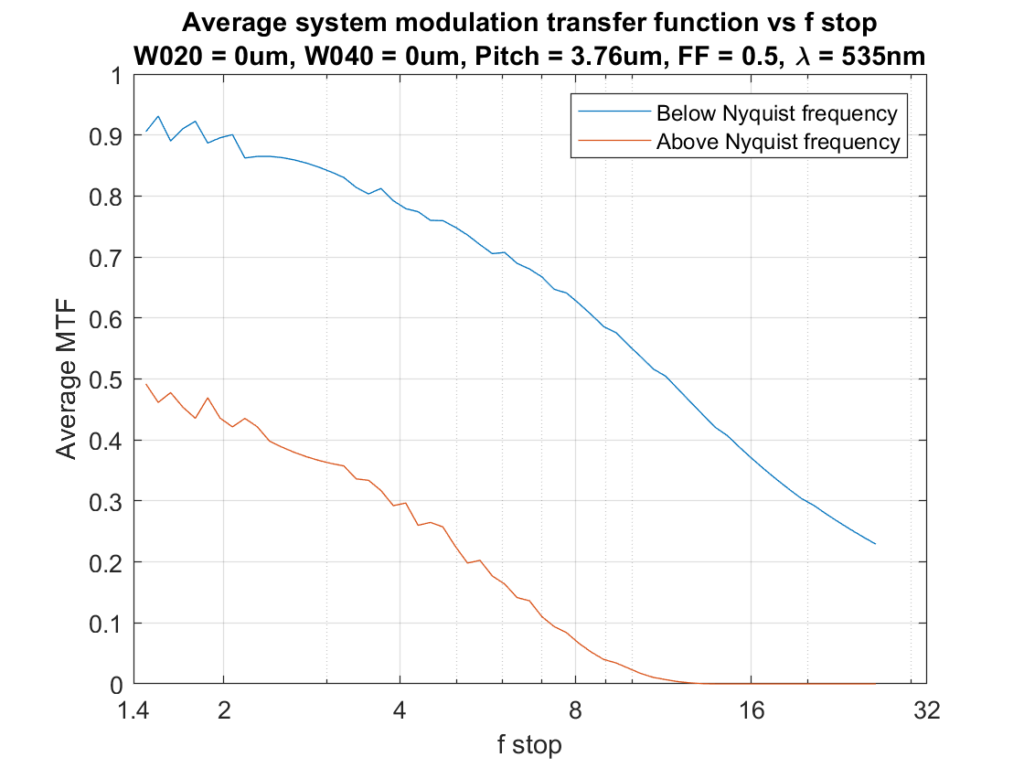
If we reduce the fill factor to about that of the GFX 50S cand GFX 50R cameras, we get a lot more aliasing and a little more sharpness:
All that is for a monochrome sensor. It would also apply to a Foveon sensor. But almost all the digital cameras use Bayer color filter arrays (CFAs). How do we modify what we’ve done to reflect that? It’s not easy. With a monochromatic target, in the right (strongly magenta) light and the right demosaicing algorithm, the monochromatic MTFs will match the ones from a Bayer CFA. The most pessimistic way of looking at things says that the sampling frequency for a Bayer-CFA sensor is half that of a monochromatic sensor with the same pixel pitch. As a rule of thumb, I favor multiplying the sensor pitch by numbers between 1.3 and 1.7. Here’s what happens at f/16 when we pick 1.5 and use that to calculate something I’ll call the effective Nyquist frequency:
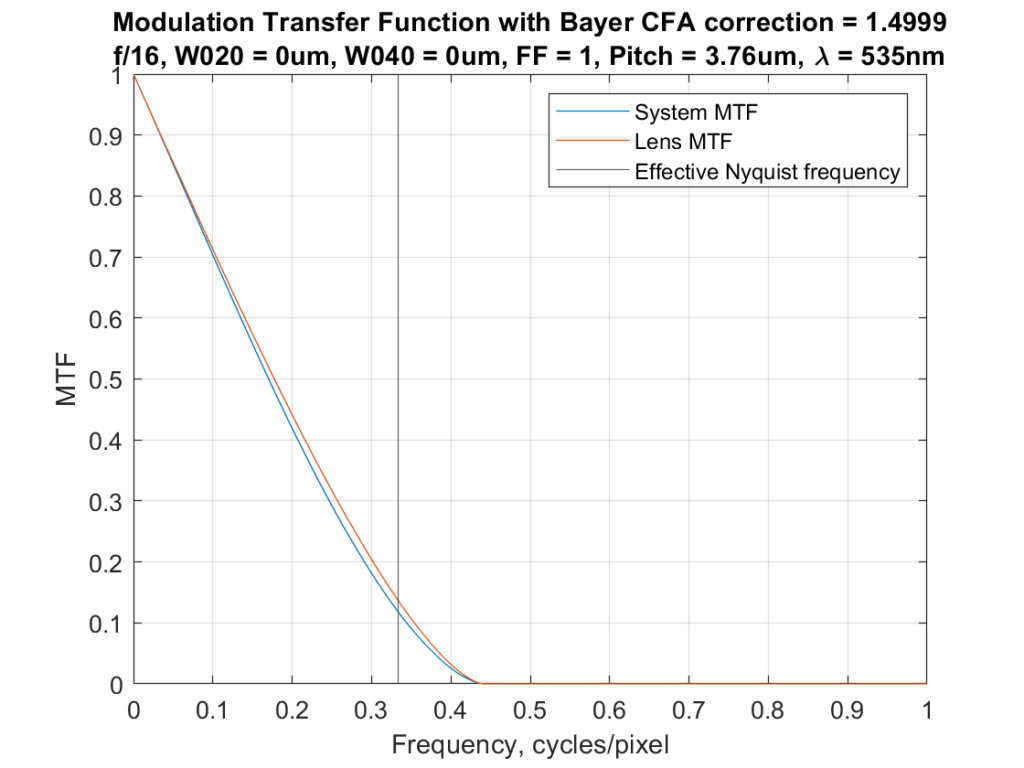
This fits fairly well with the real-world testing that I’ve done, which says that, with a good lens and a high-spatial-frequency target, there is noticeable aliasing at f/11 but the there is none speak of at f/16.
At f/4:
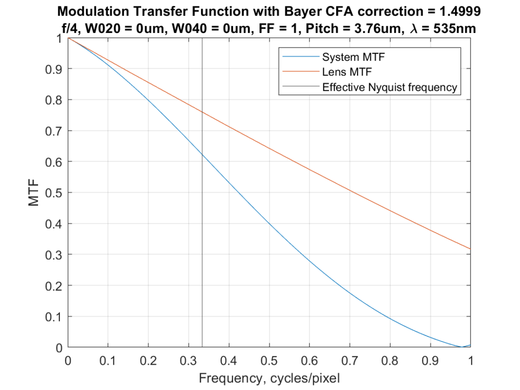
The graph shows quite a bit of energy in the System MTF above the adjusted Nyquist frequency. Although I don’t have any lenses that are diffraction-limited at f/4, my real world experience shows strong aliasing with good lenses at that aperture.
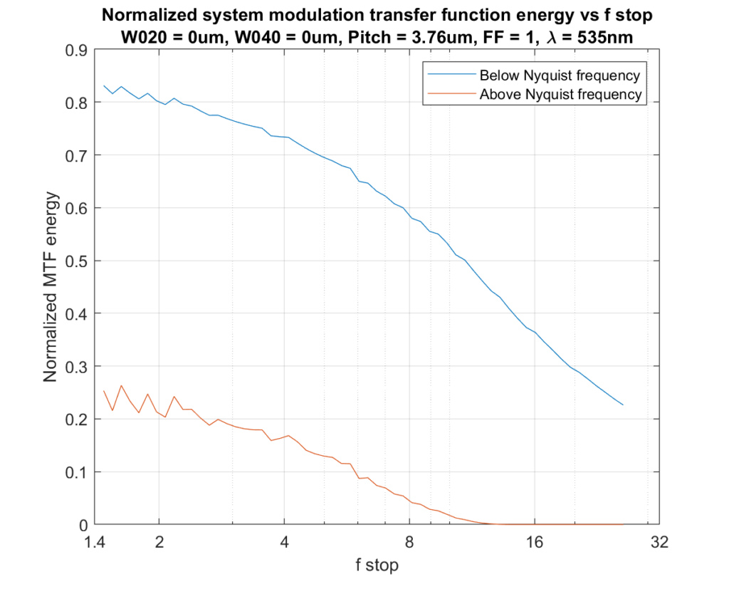
Now I’ll show you the effect of calculating the amount of energy on both sides of the Nyquist frequency for a range of f-stops. In the case of the monochromatic sensor, the numbers are the same as using the average MTFs above and below the Nyquist frequency as I did in the previous post, but I’ve had to make some changes to the definitions so that they will make sense when used with the effective Nyquist frequency. The normalized energy below the effective Nyquist frequency is the sum of all the MTFs below that frequency divided by the number of data points below that frequency, so it amounts to the average MTF. The normalized energy above the effective Nyquist frequency is the sum of all the MTFs between that frequency and one cycle per pixel divided by the same number as we used for energy below the Nyquist frequency.
Here is the result for the monochromatic case, and it’s the same as above:
And here’s what happens when a CFA correction factor of 1.5 is applied, and the effective Nyquist frequency drops to 0.33 cycles/pixel:
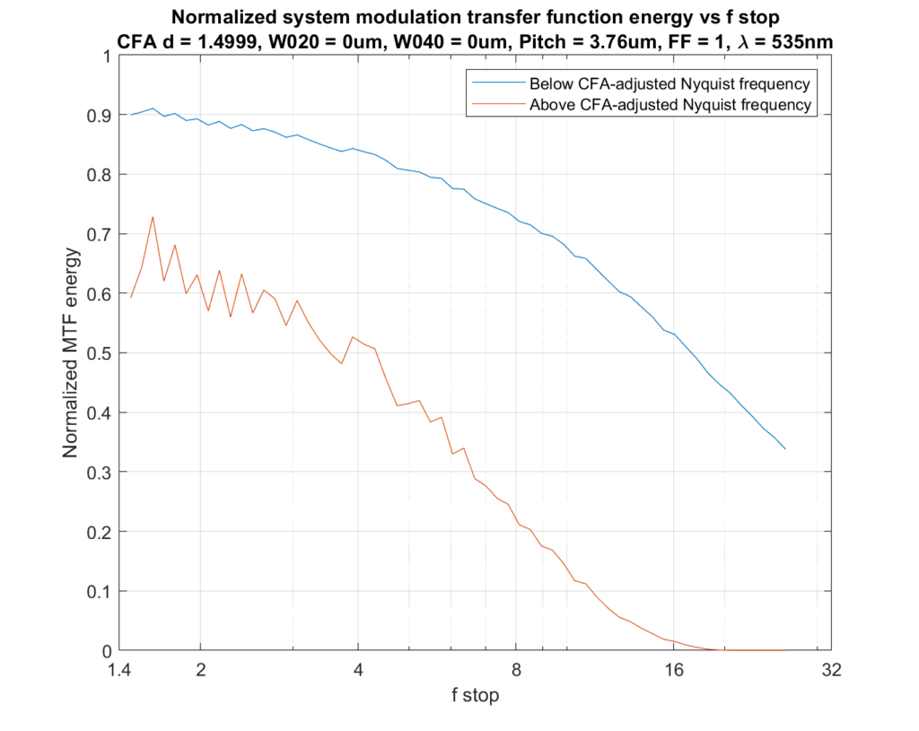
This shows aliasing ceasing to become an issue between f/11 and f/16, which matches my experience with the GFX 100 and a7RIV.
Hi Jim,
You state “I am reporting on the MTF in the vertical and horizontal direction. The MTF measured diagonally will be lower.”
I think you dropped the angular frequency scaling factors along the way. The 2D MTF of a square photosite aperture is
sinc(fx)*sinc(fy)
If you take a transect through this at an angle “theta” to produce a 1D MTF, then
fx = cos(theta)*x
fy = sin(theta)*y.
In the diagonal case, this means cos(theta)=sin(theta) ~= 0.71, which means the MTF through the diagonal will be slightly higher than the horizontal and vertical cases.
Not a problem in this article, but it is easy enough to add to your code for future use.
-F
Thanks, Frans, I’ll make the change. The error was one of conception, not of coding, since I was using numerical, not analytic methods. I never actually looked at the diagonal MTFs; I just guessed what would happen based on a longer averaging extent in that direction.