• site home
  • blog home
  • galleries
  • contact
  • underwater
  • the bleeding edge

the last word

Photography meets digital computer technology. Photography wins -- most of the time.

You are here: Home / The Last Word / Cost functions for optimal blur management

Cost functions for optimal blur management

May 1, 2019 JimK Leave a Comment

This is a continuation of a series of posts about blur management for landscape photography. The series starts here. This is quite a nerdy little post. If you aren’t interested in the mathematical details behind deciding the best way to manage blur you should probably move on.

To search for an optimum solution to a problem, you need to define a scalar (one-dimensional) metric of goodness or badness. You can maximize the goodness, or minimize the badness. When I set up the blur optimizer, I picked two such metrics, the diameter of the circle of confusion (CoC), and the number of those CoCs per picture height. The first is a measure of badness, and I’ve been posting solutions that minimize it. The second is a goodness assessment, and I haven’t posted any results that use that.

But there’s another set of decisions to me made: how the contributions to fuzziness (CoC diameter) or sharpness (CoCs/ph) are to be aggregated with respect to the distances and the weights. In everything I’ve posted so far, the diameters at each distance have been squared, then multiplied by the weights, then summed. This is the so-called “sum of squares” conversion from vector to scalar that I usually employ when I have no reason to do otherwise.

Sum of squares weights the worst cases more than better ones. I’ve noticed that in the solutions I’ve posted. But there are other, perfectly reasonable, ways of adding up the errors at the selected distances. One is to do a simple weighted sum: weight the blur diameters at each distance by the assigned weight, then just add ’em up. There’s an even simpler approach: ignore the weight, and simply minimize the worst-case blur diameter.

In this post, I’m going to show you what happens when all three are applied to an image. It’s one you’ve seen before if you’ve been following along in this series.


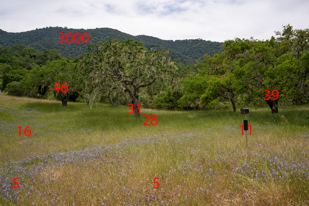
Distances in meters are labeled in red. Focal length was 30 mm . Camera was  a Nikon Z7, and I used the Nikon 14-30 mm f/4 zoom.

Here are the results of all three methods:


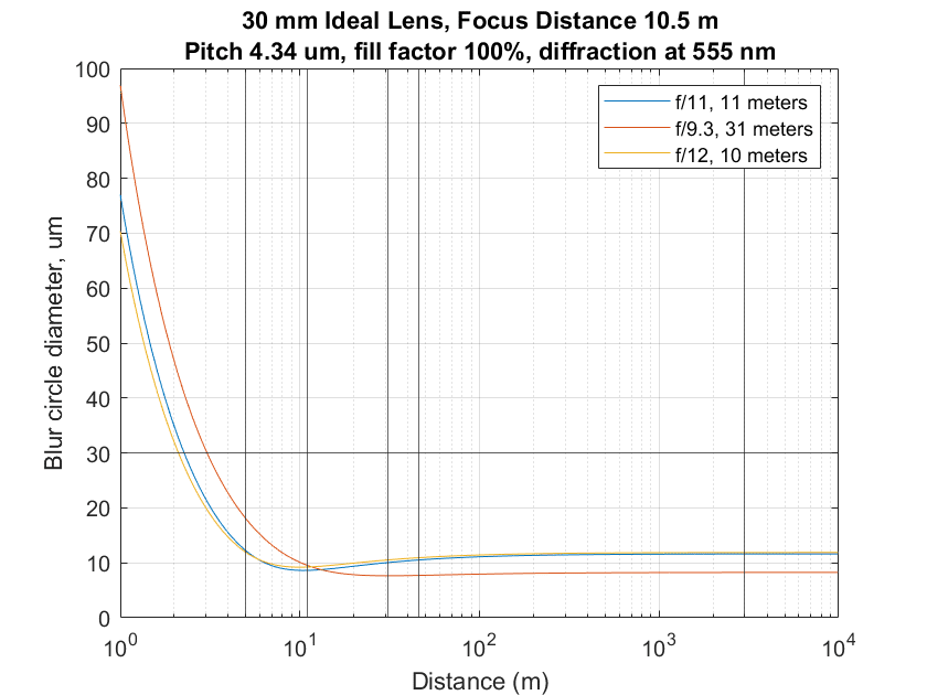
The blue curve is the one you’ve seen before. I got to that with the sum of squares approach. The red curve is the result of choosing a simple weighted sum. You can see that it is significantly more distant in its choice of where to focus, and slightly more aggressive about opening up to avoid diffraction. The yellow worst-case results are very similar to the sum of squares ones.

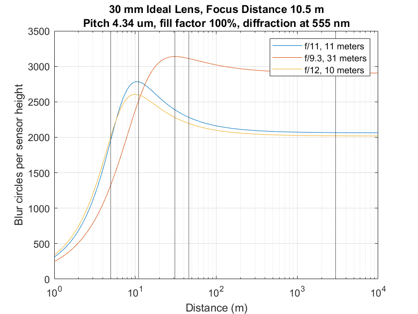
If we flip the graphs over and look at a sharpness metric, the differences where the CoCs are small become more apparent, and the deltas when the CoCs are large get visually smaller.

What’s the right answer? Depends on your objectives. I’m thinking about exploring exponents between 1 and 2.

The Last Word

← FF examples of optimal blur management Comparing blur circles across formats and sensors →

Leave a Reply Cancel reply

Your email address will not be published. Required fields are marked *

May 2025
S M T W T F S
 123
45678910
11121314151617
18192021222324
25262728293031
« Apr    

Articles

  • About
    • Patents and papers about color
    • Who am I?
  • How to…
    • Backing up photographic images
    • How to change email providers
    • How to shoot slanted edge images for me
  • Lens screening testing
    • Equipment and Software
    • Examples
      • Bad and OK 200-600 at 600
      • Excellent 180-400 zoom
      • Fair 14-30mm zoom
      • Good 100-200 mm MF zoom
      • Good 100-400 zoom
      • Good 100mm lens on P1 P45+
      • Good 120mm MF lens
      • Good 18mm FF lens
      • Good 24-105 mm FF lens
      • Good 24-70 FF zoom
      • Good 35 mm FF lens
      • Good 35-70 MF lens
      • Good 60 mm lens on IQ3-100
      • Good 63 mm MF lens
      • Good 65 mm FF lens
      • Good 85 mm FF lens
      • Good and bad 25mm FF lenses
      • Good zoom at 24 mm
      • Marginal 18mm lens
      • Marginal 35mm FF lens
      • Mildly problematic 55 mm FF lens
      • OK 16-35mm zoom
      • OK 60mm lens on P1 P45+
      • OK Sony 600mm f/4
      • Pretty good 16-35 FF zoom
      • Pretty good 90mm FF lens
      • Problematic 400 mm FF lens
      • Tilted 20 mm f/1.8 FF lens
      • Tilted 30 mm MF lens
      • Tilted 50 mm FF lens
      • Two 15mm FF lenses
    • Found a problem – now what?
    • Goals for this test
    • Minimum target distances
      • MFT
      • APS-C
      • Full frame
      • Small medium format
    • Printable Siemens Star targets
    • Target size on sensor
      • MFT
      • APS-C
      • Full frame
      • Small medium format
    • Test instructions — postproduction
    • Test instructions — reading the images
    • Test instructions – capture
    • Theory of the test
    • What’s wrong with conventional lens screening?
  • Previsualization heresy
  • Privacy Policy
  • Recommended photographic web sites
  • Using in-camera histograms for ETTR
    • Acknowledgments
    • Why ETTR?
    • Normal in-camera histograms
    • Image processing for in-camera histograms
    • Making the in-camera histogram closely represent the raw histogram
    • Shortcuts to UniWB
    • Preparing for monitor-based UniWB
    • A one-step UniWB procedure
    • The math behind the one-step method
    • Iteration using Newton’s Method

Category List

Recent Comments

  • Mike MacDonald on Your photograph looks like a painting?
  • Mike MacDonald on Your photograph looks like a painting?
  • bob lozano on The 16-Bit Fallacy: Why More Isn’t Always Better in Medium Format Cameras
  • JimK on Goldilocks and the three flashes
  • DC Wedding Photographer on Goldilocks and the three flashes
  • Wedding Photographer in DC on The 16-Bit Fallacy: Why More Isn’t Always Better in Medium Format Cameras
  • JimK on Fujifilm GFX 100S II precision
  • Renjie Zhu on Fujifilm GFX 100S II precision
  • JimK on Fuji 20-35/4 landscape field curvature at 23mm vs 23/4 GF
  • Ivo de Man on Fuji 20-35/4 landscape field curvature at 23mm vs 23/4 GF

Archives

Copyright © 2025 · Daily Dish Pro On Genesis Framework · WordPress · Log in

Unless otherwise noted, all images copyright Jim Kasson.