This is a continuation of a report on new ways to look at depth of field. The series starts here:
The shape of the curves. Let’s take a closer look at the DOF curves for the simulated Otus lens focused at three meters that I showed in the first part of this summary:
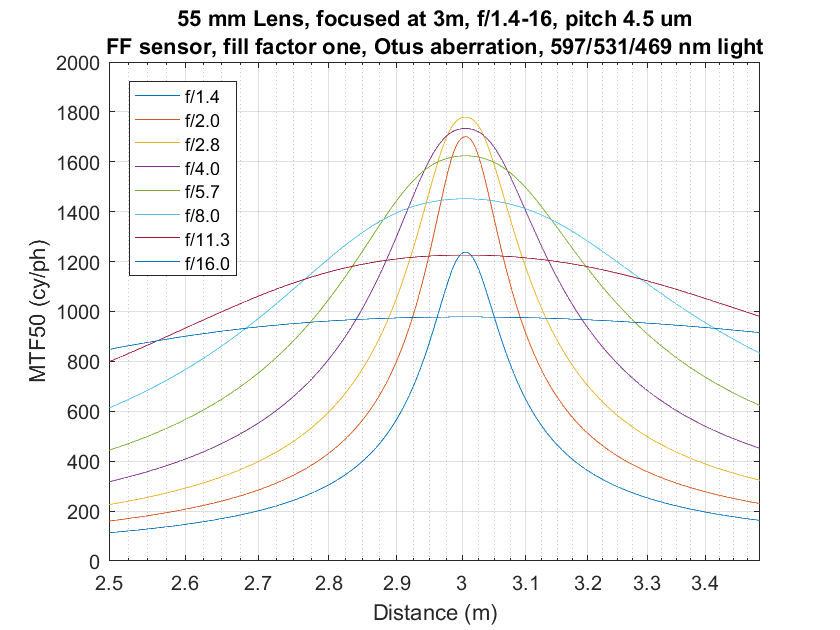
I already remarded on how narrow the really sharp parts are at wide apertures. Now I’d like to direct your attention to the shape of the curves. They are in general, bell-shaped, like the probability density function of a Gaussian distribution. From a DOF perspective, that means that there’s a region where the curves are flatter near the focus point meaning things are pretty sharp. If you get away from that region, the curves fall away steeply, meaning the image gets real soft real fast. And finally, when the object that you’re looking at gets quite far from the point of focus, distance stops making so much difference in the sharpness. That’s the good news. The bad news is that the image is getting pretty darned soft by then.
Sharp lenses have less relative DOF at the same f-stop, but there’s a workaround that reverses the situation. Consider these three sets of curves with three different lenses focused at 3 meters:
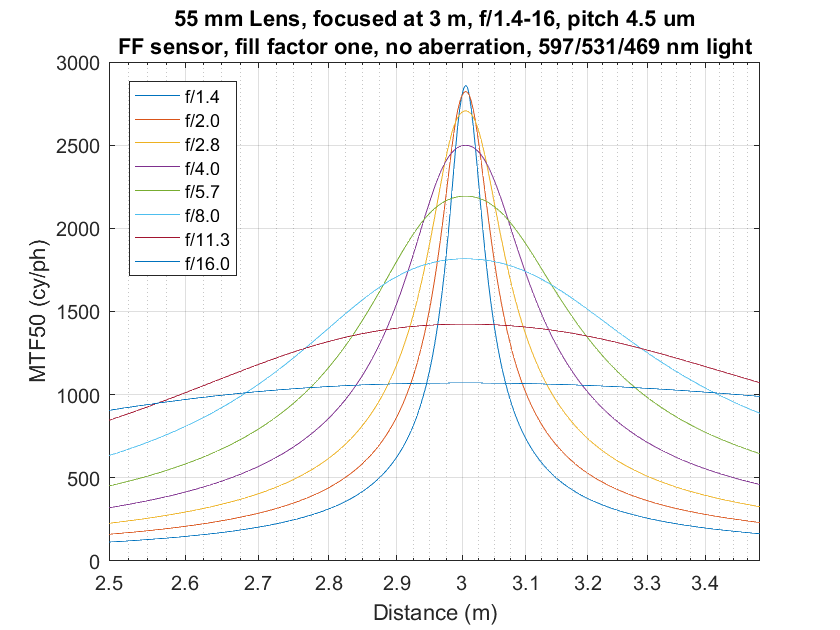
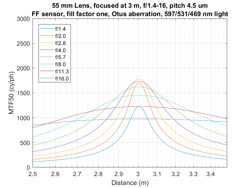
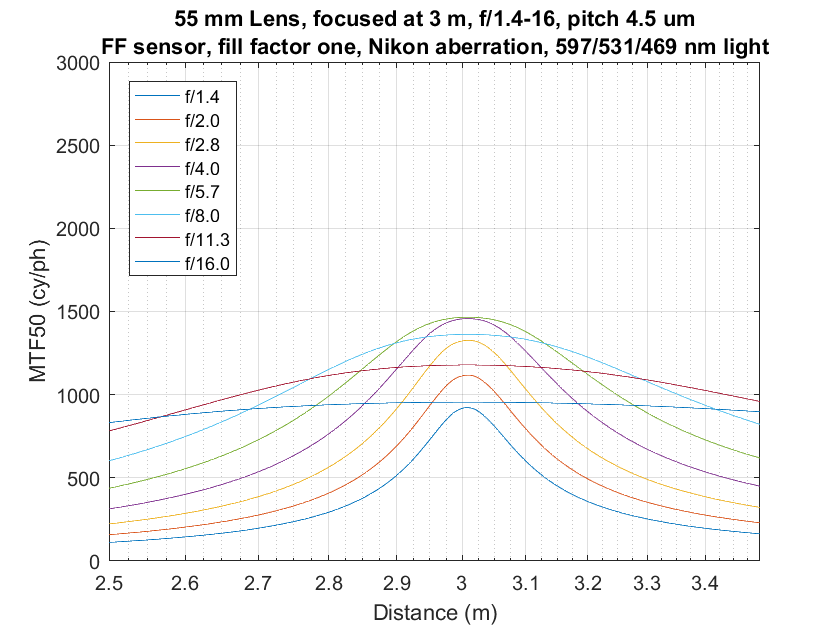
The top set of curves is for an ideal, diffraction-limited lens on a Sony a7RII. The next set down is for a 55mm lens with the same aberrations as the 85/1.4 Otus. The bottom set is for a 55mm lens with the same aberrations as the 85/1.4G Nikon.
You can see that, at the wider apertures where diffraction isn’t the long pole in the tent, that the better the lens, the peakier and narrower are the curves. I wish it weren’t that way, but if you wan the sharpness your fancy lens was made to deliver, you’re going to have to find flatter subjects than you would if you were using a lesser lens.
Here’s the workaround. Just stop down a bit more. You can see that the diffraction limited lens at f/5.6 has more DOF than the other lenses at apertures that are nearly as sharp. It’s a close call, but it looks like that’s true at f/8, too.
The same kind of thing is true for the Otus and the Nikon, considered as a pair. The Otus at f/8 is almost as sharp as the Nikon at f/4 and f/5.6, and has more DOF.
Of course, the downside is that you don’t get the center sharpness you’d have gotten if you opened the good lens up farther.
Thanks. I find these bell-shaped charts more comprehensible than what I may in error have described at “extinction graphs”.
Guess? Are they more or less equivalent to one side of the bell-shaped curve? Or am I “unclear on the concept” yet again?
Also, I’m curious why you picked the Otus 55 for these simulations rather than another lens. (sorry if that was explained in a previous blog article).
I actually modeled the Otus sim on the Otus 85, and scaled it to 55mm. I picked the Otus because it’s the sharpest lens I have.
I figured that might be the reason.
Perhaps something to consider: use a more commonly available lens like the FE55 that people can relate to. I kind of “tune out” articles with the Otus since I have nothing in its class of IQ. I’m reluctant to extrapolate.
OT? Do you happen to have the FE28 f/2 and perhaps the time and interest to put it through some of the tests you do? I’d guess it is the most commonly owned native lens due to its relative affordability … at least until the FE50 joined the lens lineup?
OT*2: If you have the FE55 and FE50, it would be interesting to see the TLW / Kasson treatment on those.
If you want to look at a more ordinary lens, a cut below the Zony 55, look at the Nikon curves.
I don’t have that lens.
I don’t have the 50 FE. Sorry.
Jim
More or less. The only difference is the focused and object distance chosen, and the fact that objects can’t be further away than infinity, and it makes no sense to focus beyond infinity (although you can do it).
Duh on my part. Thanks for the explanation. Comprehension of charts in among my “senior moments”.
What would be a better term for what I describe as “extinction charts / graphs”?
FWIW:
IIRC back when school kids took a whole battery of aptitude/IQ tests, “spatial visualization” was by far my weakest aptitude. Or maybe that test was part of admission to some college program or grant?
TMI, but I am not only a mediocre chess player who plateaued quickly, but a poor checkers player.
I can just barely visualize what the board will look like after a turn or two.
TMI * 2:
My fraternal twin brother was a (or the?) collegiate champion in bridge decades ago, but I am mediocre at best after plateau’ing, even though I love the game. My speculation is that his scores for “spatial visualization” would be off the chart.
MTF50 vs object distance? Defocused MTF50? Defocused sharpness?
Jim
Jim
I can’t say that I love the graphs or charts. I went to Merkinger’s paper where he boils his what to do for maximum depth of field to: focus on infinity and stop down to a small enough F-stop to cover the smallest detail one wants to resolve.
The question I still don’t see a clear and present answer to is where to focus the camera. The vague one-third the way into the scene, the infinity focus solution, the seat of the pants explanations leave me at least completely befuddled. Having used a view camera for thirty years I could deliver a sharp image in less than two minutes and I could teach someone the two minute drill in twenty minutes. Not so with a fixed back and lens.
Call me stupid but can you give us where you focus the camera for maximum depth of field.
Thanks
The conventional answer to that is at the hyperfocal distance. I have a new way to look at the hyperfocal distance, but the principle still applies. However, if you do this, you’re gonna guarantee that objects at infinity are at whatever you decided was your minimal acceptable sharpness, which is not what is best for many scenes.
In a situation like that, I’d ask myself what MTF50 at infinity is desirable, and use that to find the hyperfocal distance. Unfortunately, at this point, I can’t tell you how to calculate that without simulating your camera and lens.
I’m still thinking about how to make this practical.
Jim
Jim
I think that looking at this from a practical perspective might be helpful. With a 50 mm lens with a depth of field from 4 feet to 50 feet where would one place the plane of focus stopping down to f 16. 4 feet to 300 feet. 4 feet to infinity.
The other discussion that’s important is what can sharpening accomplish.
The other part of the discussion that’s pertinent is how this all looks in a 30×40 print. Proof is in the pudding in my book.
I can make prints, but using what for a subject? Is there some subject that everybody agrees is relevant to their work? I think not.
And if I make the prints, how can I show them to you?
I think the printmaking is something that you should do for yourself.
Jim
This may be the wrong web site for you.
[Added later, after a comment about the possibility that I was offended by your comment:
I’m not at all offended. I know graphs and charts aren’t for everyone. I’m simply saying that if they’re not for you, than this graph and chart heavy web site is probably a bad fit.]
Jim