the last word

Photography meets digital computer technology. Photography wins -- most of the time.

  • site home
  • blog home
  • galleries
  • contact
  • underwater
  • the bleeding edge
You are here: Home / Color Science / Dimensionality of patch sets and natural spectra

Dimensionality of patch sets and natural spectra

April 17, 2022 JimK Leave a Comment

A DPR PS&T member kindly supplied me with a collection of reflectance spectra about 220 natural objects. I added that set to my other patch sets, and performed a principal component analysis (PCA) on each set. One thing I did differently this time is I restricted the wavelengths under consideration to the set between 400 and 700 nm, inclusive. That provided a more level playing field, since I had values in that range for all the sets.

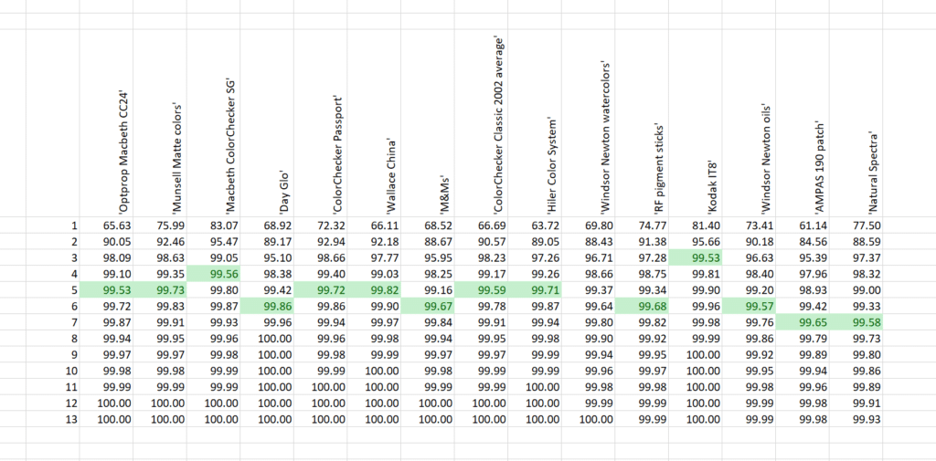
The top row contains descriptors of the patch sets. The first column is the number of eigenvectors used in the reconstruction. The rest of the readings are the cumulative “explained” metric of PCA, which, for n in column 1, is the percentage of the total variance explained by the eigenvectors from 1 through n. I’ve flagged the first place in each column where the score is above 99.5%.

The set with the lowest dimensionality is the Kodak IT8 set. That makes sense, since that set was created from one set of three film dyes. The patch set with the highest dimensionality is the AMPAS 190-patch set, but the natural spectra set has slightly higher dimensionality.

Another way to look at it is to subtract the “explained” field from 100, to give a metric of residual error:

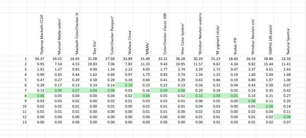
I’ve identified in green the number of eigenvectors it took to drop the residual error to 0.1 or less.

Graphically:

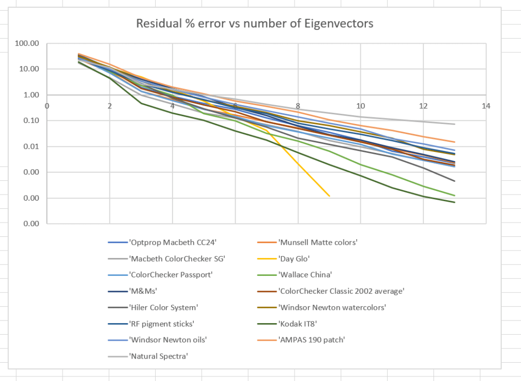
It looks like 12 eigenvectors is enough for this set of real world reflectance spectra, which is heavily biased towards botanical objects.


Color Science, The Last Word

← Training on the ColorCheckers, testing on natural spectra Natural colors — reflectance spectra metamers →

Leave a Reply Cancel reply

Your email address will not be published. Required fields are marked *

February 2023
S M T W T F S
 1234
567891011
12131415161718
19202122232425
262728  
« Jan    

Articles

  • About
    • Patents and papers about color
    • Who am I?
  • Good 35-70 MF lens
  • How to…
    • Backing up photographic images
    • How to change email providers
  • Lens screening testing
    • Equipment and Software
    • Examples
      • Bad and OK 200-600 at 600
      • Excellent 180-400 zoom
      • Fair 14-30mm zoom
      • Good 100-200 mm MF zoom
      • Good 100-400 zoom
      • Good 100mm lens on P1 P45+
      • Good 120mm MF lens
      • Good 18mm FF lens
      • Good 24-105 mm FF lens
      • Good 24-70 FF zoom
      • Good 35 mm FF lens
      • Good 60 mm lens on IQ3-100
      • Good 63 mm MF lens
      • Good 65 mm FF lens
      • Good 85 mm FF lens
      • Good and bad 25mm FF lenses
      • Good zoom at 24 mm
      • Marginal 18mm lens
      • Marginal 35mm FF lens
      • Mildly problematic 55 mm FF lens
      • OK 16-35mm zoom
      • OK 60mm lens on P1 P45+
      • OK Sony 600mm f/4
      • Pretty good 16-35 FF zoom
      • Pretty good 90mm FF lens
      • Problematic 400 mm FF lens
      • Tilted 20 mm f/1.8 FF lens
      • Tilted 30 mm MF lens
      • Tilted 50 mm FF lens
      • Two 15mm FF lenses
    • Found a problem – now what?
    • Goals for this test
    • Minimum target distances
      • MFT
      • APS-C
      • Full frame
      • Small medium format
    • Printable Siemens Star targets
    • Target size on sensor
      • MFT
      • APS-C
      • Full frame
      • Small medium format
    • Test instructions — postproduction
    • Test instructions — reading the images
    • Test instructions – capture
    • Theory of the test
    • What’s wrong with conventional lens screening?
  • Previsualization heresy
  • Privacy Policy
  • Recommended photographic web sites
  • Using in-camera histograms for ETTR
    • Acknowledgments
    • Why ETTR?
    • Normal in-camera histograms
    • Image processing for in-camera histograms
    • Making the in-camera histogram closely represent the raw histogram
    • Shortcuts to UniWB
    • Preparing for monitor-based UniWB
    • A one-step UniWB procedure
    • The math behind the one-step method
    • Iteration using Newton’s Method

Category List

Recent Comments

  • Brian Olson on Fuji GFX 100S exposure strategy, M and A modes
  • JimK on Picking a macro lens
  • JimK on Picking a macro lens
  • Glenn Whorrall on Picking a macro lens
  • JimK on What pitch do you need to scan 6×6 TMax 100?
  • Hatzipavlis Peter on What pitch do you need to scan 6×6 TMax 100?
  • JeyB on Internal focusing 100ish macro lenses
  • JimK on How focus-bracketing systems work
  • Garry George on How focus-bracketing systems work
  • Rhonald on Format size and image quality

Archives

Copyright © 2023 · Daily Dish Pro On Genesis Framework · WordPress · Log in

Unless otherwise noted, all images copyright Jim Kasson.