• site home
  • blog home
  • galleries
  • contact
  • underwater
  • the bleeding edge

the last word

Photography meets digital computer technology. Photography wins -- most of the time.

You are here: Home / The Last Word / Getting to the point of best focus from raw MTF50 curves

Getting to the point of best focus from raw MTF50 curves

March 4, 2016 JimK 8 Comments

When you focus using the LCD screen or an attached monitor, with or without the peaking enabled, you are focusing on luminance. And that’s appropriate, since human contrast sensitivity functions allow us to see fine image detail by seeing changes in luminance.

But I’ve been reporting on the peaks in raw color planes. How does that relate to luminance peaks? Jack Hogan took some of my test images, examined them, and came up with a set of raw plane weightings to get luminance or CIE 1931 Y.

That’s nice. But does it help us take the three raw MTF50 curves and predict the point of best focus? Let’s try a crude experiment.  Applying Jack’s weighting vector – [0.93 1.0 0.1142] – to the MTF50 curves gives us the black curve in the following plot:

lum mtf50 calculated r

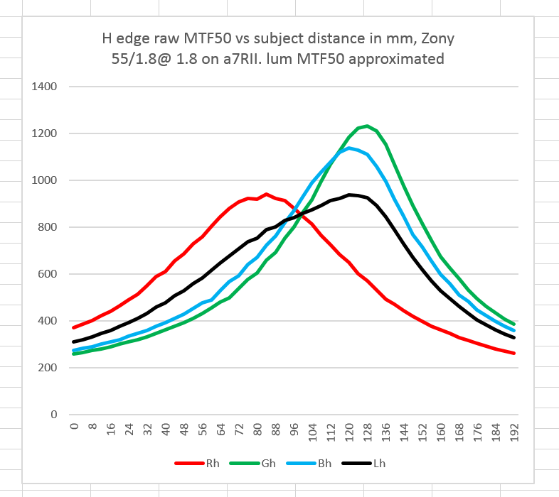
Doesn’t look very credible, does it?

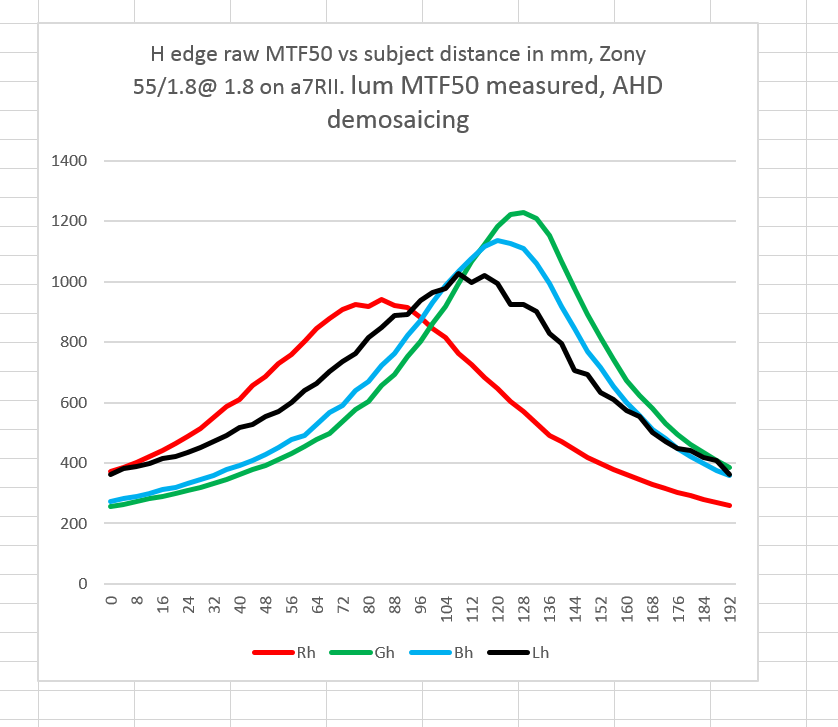
If we use DCRAW with the AHD option selected to demosaic the same set of files, and also let DCRAW do the white balancing with the -a option, then have Imatest compute the MTF50s, we get this:

lum mtf50 measured r

Back to the drawing board…

We can salvage some things from this experiment.

It does look as though Jack’s weighting vector is about right. It looks like, as you would expect, the blue raw plane has little to do with the point of best focus, and that the point of best focus lies about halfway between the red plane peak and the green plane peak, but biased a little towards the green plane peak.

That’s with the target illuminated with a 5000K light source. A lower numeric color temperature would make the red plane relatively more important.


The Last Word

← Another medium tele test — Batis AF vs MF Another medium tele test — Bokeh →

Comments

  1. Erik Kaffehr says

    March 4, 2016 at 9:43 pm

    Jim,

    Lot of interesting stuff! All was pretty obvious before you started looking into it, wasn’t it?

    Best regards
    Erik

    Reply
    • Jim says

      March 5, 2016 at 7:03 am

      Erik, it’s a surprise to me how much the red raw channel affects the luminance MTF50 curve. Obvious in retrospect, of course, but a lot of things are.

      Jim

      Reply
  2. Jack Hogan says

    March 5, 2016 at 12:53 am

    The demosaiced curve ‘looks’ better, assuming I did not make any mistakes. Is it better? In theory the difference is a Bradford transformation to D65 and a matrix to sRGB (I assume) and gamma. Gamma I would exclude because it is supposed to be undone by the output medium.

    So should we go to linear sRGB for a better correlate to perceptual sharpness? In other words, where should we stop? Input referred, PCS, or output referred? We know that in theory Y in XYZ is proportional to Luminance in cd/m^2, and that’s what the eye sees in nature. What coefficients were used by Imatest to convert sRGB to the ‘luminance’ channel? Isn’t that ‘luminance’ just an approximation of the more precise linear Luminance in Y which is proportional to the actual photometric quantity that hit the sensor?

    Jack

    Reply
    • Jack Hogan says

      March 5, 2016 at 5:52 am

      Also, reading MTF Mapper’s documentation the first thing it does is linearize and convert a color image to grayscale by 0.299R + 0.587G + 0.114B. I assume Imatest does something similar. This makes me feel even more comfortable with sticking to the PCS or earlier for the weights.

      Reply
      • Frans van den Bergh says

        March 7, 2016 at 10:47 pm

        Correct. If necessary (say, for custom channel weights), images could be mixed down from RGB to grayscale before feeding them to MTF Mapper (for now).

        I suppose that there are two possible enhancements to facilitate these colour space experiments:
        1. Allow custom R,G,B weights to be passed to MTF Mapper, or
        2. Try to extract colour profile information from the input image. This could be tricky, but if the input image is a .tif, .jpg or a .png, the format could provide us with more detailed colour space information. How to use this information to produce a better monochromatic image is something I will have to research first.

        Reply
    • Jim says

      March 5, 2016 at 7:05 am

      The demosaiced curve ‘looks’ better, assuming I did not make any mistakes. Is it better? In theory the difference is a Bradford transformation to D65 and a matrix to sRGB (I assume) and gamma. Gamma I would exclude because it is supposed to be undone by the output medium.

      Imatest takes the gamma into account. So consider that calibrated out.

      Jim

      Reply
      • Frans van den Bergh says

        March 7, 2016 at 10:39 pm

        MTF Mapper tries to guess what to do about gamma correction, which boils down to the following heuristics:
        1. If the input image has a bit depth of 16, then the image is assumed to be linear,
        2. If the input image has a bit depth of 8, it assumes that the values are encoded in sRGB gamma, and it applies the inverse to produce a linear 16-bit image internally for further processing.
        3. If the “-l” option is specified, then 8-bit images are assumed to be linear, and are simply scaled to 16 bits internally.

        The implied assumption here being that 8-bit images could be JPEGs (although no explicit checks are performed), and that linear 8-bit images are rare. If there are reasonable checks that can be performed (i.e., without having to perform too much low-level image format specific work) without making any assumptions regarding the contents of the image, I would certainly be willing to implement them.

        Reply
    • Jim says

      March 5, 2016 at 7:08 am

      So should we go to linear sRGB for a better correlate to perceptual sharpness?

      The best stand-in we have for sensory response to luminance is L* which is Y^(1/3) with a straight line near zero. However, since the noniinearity is monotonic, it won’t change the location of the peaks.

      Jim

      Reply

Leave a Reply Cancel reply

Your email address will not be published. Required fields are marked *

May 2025
S M T W T F S
 123
45678910
11121314151617
18192021222324
25262728293031
« Apr    

Articles

  • About
    • Patents and papers about color
    • Who am I?
  • How to…
    • Backing up photographic images
    • How to change email providers
    • How to shoot slanted edge images for me
  • Lens screening testing
    • Equipment and Software
    • Examples
      • Bad and OK 200-600 at 600
      • Excellent 180-400 zoom
      • Fair 14-30mm zoom
      • Good 100-200 mm MF zoom
      • Good 100-400 zoom
      • Good 100mm lens on P1 P45+
      • Good 120mm MF lens
      • Good 18mm FF lens
      • Good 24-105 mm FF lens
      • Good 24-70 FF zoom
      • Good 35 mm FF lens
      • Good 35-70 MF lens
      • Good 60 mm lens on IQ3-100
      • Good 63 mm MF lens
      • Good 65 mm FF lens
      • Good 85 mm FF lens
      • Good and bad 25mm FF lenses
      • Good zoom at 24 mm
      • Marginal 18mm lens
      • Marginal 35mm FF lens
      • Mildly problematic 55 mm FF lens
      • OK 16-35mm zoom
      • OK 60mm lens on P1 P45+
      • OK Sony 600mm f/4
      • Pretty good 16-35 FF zoom
      • Pretty good 90mm FF lens
      • Problematic 400 mm FF lens
      • Tilted 20 mm f/1.8 FF lens
      • Tilted 30 mm MF lens
      • Tilted 50 mm FF lens
      • Two 15mm FF lenses
    • Found a problem – now what?
    • Goals for this test
    • Minimum target distances
      • MFT
      • APS-C
      • Full frame
      • Small medium format
    • Printable Siemens Star targets
    • Target size on sensor
      • MFT
      • APS-C
      • Full frame
      • Small medium format
    • Test instructions — postproduction
    • Test instructions — reading the images
    • Test instructions – capture
    • Theory of the test
    • What’s wrong with conventional lens screening?
  • Previsualization heresy
  • Privacy Policy
  • Recommended photographic web sites
  • Using in-camera histograms for ETTR
    • Acknowledgments
    • Why ETTR?
    • Normal in-camera histograms
    • Image processing for in-camera histograms
    • Making the in-camera histogram closely represent the raw histogram
    • Shortcuts to UniWB
    • Preparing for monitor-based UniWB
    • A one-step UniWB procedure
    • The math behind the one-step method
    • Iteration using Newton’s Method

Category List

Recent Comments

  • bob lozano on The 16-Bit Fallacy: Why More Isn’t Always Better in Medium Format Cameras
  • JimK on Goldilocks and the three flashes
  • DC Wedding Photographer on Goldilocks and the three flashes
  • Wedding Photographer in DC on The 16-Bit Fallacy: Why More Isn’t Always Better in Medium Format Cameras
  • JimK on Fujifilm GFX 100S II precision
  • Renjie Zhu on Fujifilm GFX 100S II precision
  • JimK on Fuji 20-35/4 landscape field curvature at 23mm vs 23/4 GF
  • Ivo de Man on Fuji 20-35/4 landscape field curvature at 23mm vs 23/4 GF
  • JimK on Fuji 20-35/4 landscape field curvature at 23mm vs 23/4 GF
  • JimK on Fuji 20-35/4 landscape field curvature at 23mm vs 23/4 GF

Archives

Copyright © 2025 · Daily Dish Pro On Genesis Framework · WordPress · Log in

Unless otherwise noted, all images copyright Jim Kasson.