• site home
  • blog home
  • galleries
  • contact
  • underwater
  • the bleeding edge

the last word

Photography meets digital computer technology. Photography wins -- most of the time.

You are here: Home / The Last Word / Noise effects of Photoshop Bicubic Sharper downsizing

Noise effects of Photoshop Bicubic Sharper downsizing

September 23, 2014 JimK Leave a Comment

Same test image as yesterday 4000×4000 monochromatic, 16-bit gray gamma 2.2, filled with a constant signal of half-scale, (0.5, 127.5, or 32767.5, depending on how you think of it), with Gaussian noise with standard deviation of 1/10 scale added to it. The image was created in Matlab, written out as a 16-bit TIFF, read into Photoshop, downsized by various amounts using Bicubic Sharper interpolation, exported as a 16-bit TIFF, read back into Matlab, and analyzed there.

RMS noise, aka standard deviation, of the downsampled images as measured in gray gamma 2.2:

rmsnoisePsbicubicShGraph

As in the case of bilinear interpolation, the Photoshop results are dramatically different than the Matlab ones; in this case the standard of comparison that I’m using in Matlab is simple bicubic, since there is no algorithm for imresize called “bicubic sharper”, If you look at it with a set of orange dots indicating “perfect” results, you can see we’re pretty close:

rmsnoisePsbicubicShWperfect

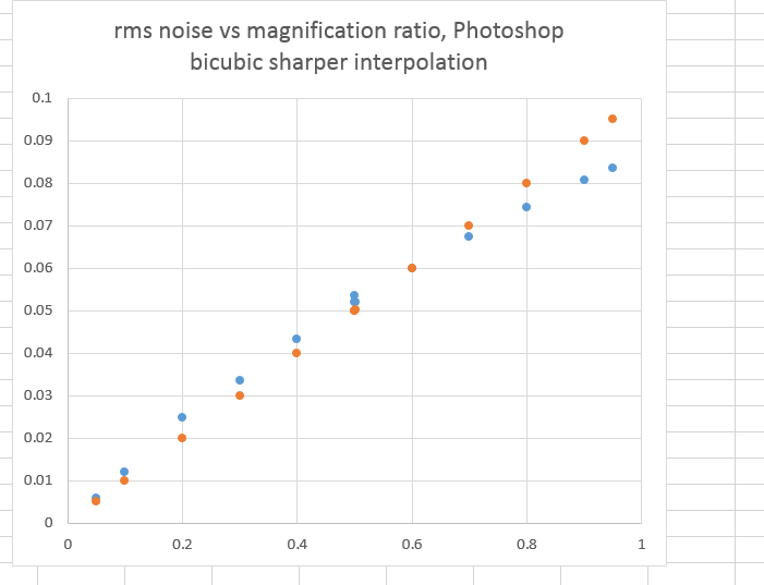
A little worse at low reduction ratios, a little better from 1/8 to 1/2. There’s a strange anomaly around 1/2 — both 0.501 and 0.499 have slightly less noise than 0.500 — but that’s hardly worth worrying about, since a look at the spectra of all three indicate that they’re very similar.

And, speaking of spectra, if we look at a few, we can see that bicubic sharper gets its exemplary noise reduction properties by attenuating the highest spacial frequency signals. It needs to do something there, since it boosts signals slightly below those.

BiCuS95pct

BiCuS90pct

BiCuS80pct

BiCuS70pct

BiCuS60pctBiCuS50pct

BiCuS4pct

BiCuS30pct

BiCuS20pct

BiCuS10pct

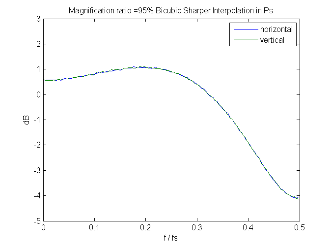
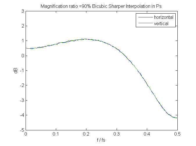
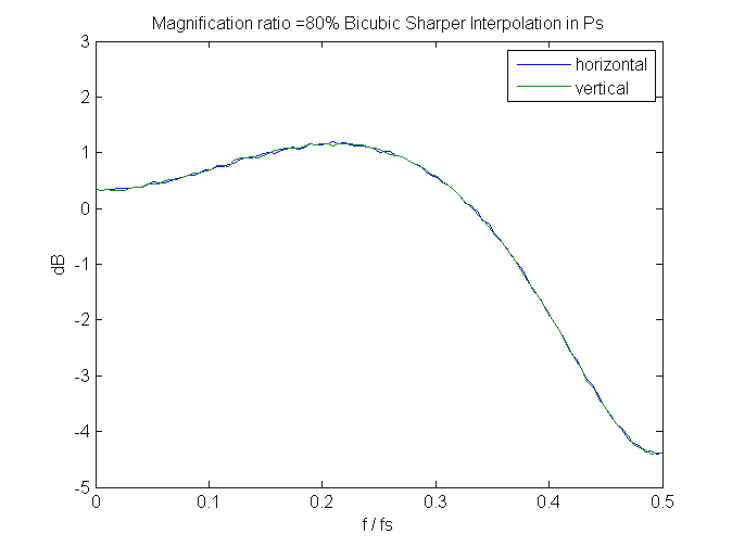
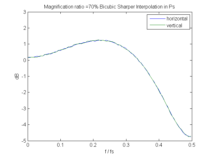
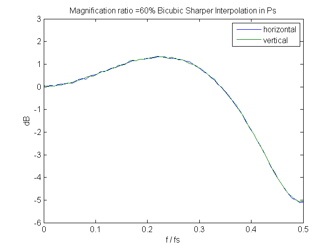
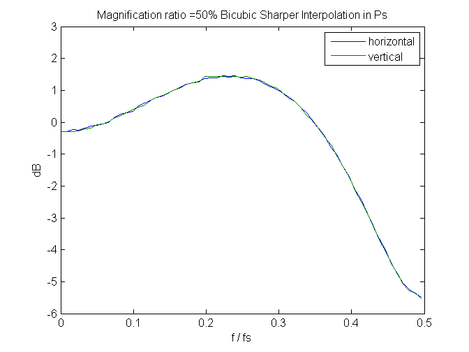
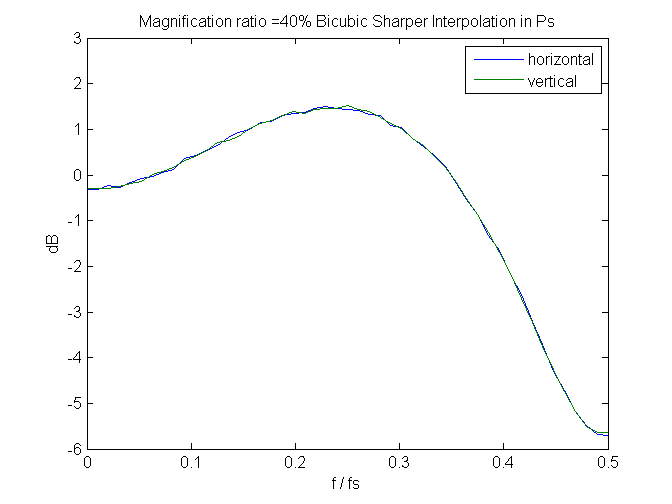
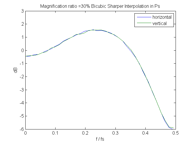
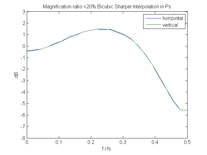
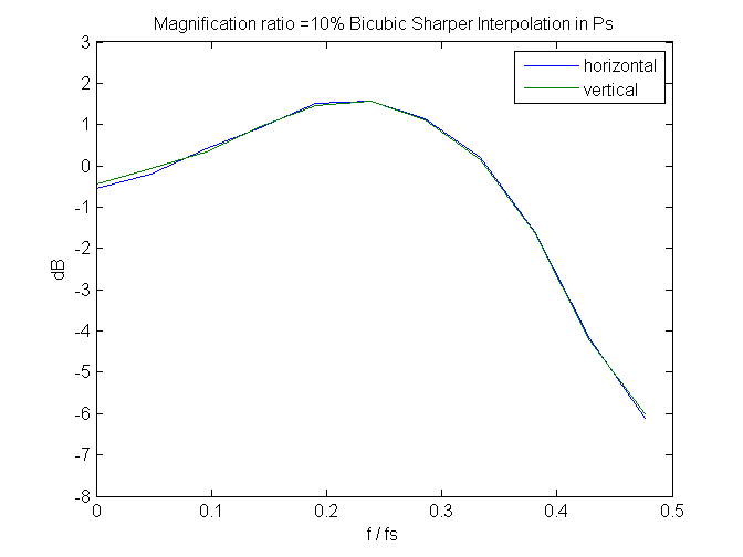
Since these are measured in the frequency domain of the output image, perfect behavior would be that the spectra don’t change with magnification. We don’t get that; greater downsampling (lower magnification) results in higher peaks and sharper cuts. Still, it’s not bad, if you don’t mind giving up that last octave of sharpness.

The Last Word

← Noise effects of Photoshop bilinear interpolation downsizing Noise effects in Lightroom downsized exporting →

Leave a Reply Cancel reply

Your email address will not be published. Required fields are marked *

July 2025
S M T W T F S
 12345
6789101112
13141516171819
20212223242526
2728293031  
« Jun    

Articles

  • About
    • Patents and papers about color
    • Who am I?
  • How to…
    • Backing up photographic images
    • How to change email providers
    • How to shoot slanted edge images for me
  • Lens screening testing
    • Equipment and Software
    • Examples
      • Bad and OK 200-600 at 600
      • Excellent 180-400 zoom
      • Fair 14-30mm zoom
      • Good 100-200 mm MF zoom
      • Good 100-400 zoom
      • Good 100mm lens on P1 P45+
      • Good 120mm MF lens
      • Good 18mm FF lens
      • Good 24-105 mm FF lens
      • Good 24-70 FF zoom
      • Good 35 mm FF lens
      • Good 35-70 MF lens
      • Good 60 mm lens on IQ3-100
      • Good 63 mm MF lens
      • Good 65 mm FF lens
      • Good 85 mm FF lens
      • Good and bad 25mm FF lenses
      • Good zoom at 24 mm
      • Marginal 18mm lens
      • Marginal 35mm FF lens
      • Mildly problematic 55 mm FF lens
      • OK 16-35mm zoom
      • OK 60mm lens on P1 P45+
      • OK Sony 600mm f/4
      • Pretty good 16-35 FF zoom
      • Pretty good 90mm FF lens
      • Problematic 400 mm FF lens
      • Tilted 20 mm f/1.8 FF lens
      • Tilted 30 mm MF lens
      • Tilted 50 mm FF lens
      • Two 15mm FF lenses
    • Found a problem – now what?
    • Goals for this test
    • Minimum target distances
      • MFT
      • APS-C
      • Full frame
      • Small medium format
    • Printable Siemens Star targets
    • Target size on sensor
      • MFT
      • APS-C
      • Full frame
      • Small medium format
    • Test instructions — postproduction
    • Test instructions — reading the images
    • Test instructions – capture
    • Theory of the test
    • What’s wrong with conventional lens screening?
  • Previsualization heresy
  • Privacy Policy
  • Recommended photographic web sites
  • Using in-camera histograms for ETTR
    • Acknowledgments
    • Why ETTR?
    • Normal in-camera histograms
    • Image processing for in-camera histograms
    • Making the in-camera histogram closely represent the raw histogram
    • Shortcuts to UniWB
    • Preparing for monitor-based UniWB
    • A one-step UniWB procedure
    • The math behind the one-step method
    • Iteration using Newton’s Method

Category List

Recent Comments

  • Jonby on How focus-bracketing systems work
  • JimK on Of fidelity, photography, audio, and wine
  • JimK on Of fidelity, photography, audio, and wine
  • AVN on Of fidelity, photography, audio, and wine
  • Markus on In photography, and in life, work and joy can, and should, coexist
  • JimK on Fuji 120/4 GF at 1:1 with tubes — visuals
  • Christopher Roberton on Fuji 120/4 GF at 1:1 with tubes — visuals
  • Pieter Kers on Visualising lens aberrations — one at a time, Siemens Star
  • JimK on Visualizing aberrations — caveats
  • Stepan Kana on Visualizing aberrations — caveats

Archives

Copyright © 2025 · Daily Dish Pro On Genesis Framework · WordPress · Log in

Unless otherwise noted, all images copyright Jim Kasson.