Observer metameric error in simulated cameras

In a previous post, I described how I had created a Matlab program to analyze sets of reflectance spectra, generate basis functions, and then use those basis functions to produce metamer sets, all with an arbitrary fixed color. For review, here is the methodology I used:

1. Using principal component analysis, find a set of basis functions for the sample set
2. Assuming the set is lit with a particular illuminant (I used D50 for the data I’m presenting here), find as many spectra as you specify by combining the basis functions.
3. All of the spectra will resolve to the same color for a CIE 1931 2-degre observer. They are therefore metamers.
4. I set the boundary conditions to exclude spectra with over 100% or less than 0%  reflectance.

I set up my camera simulator to allow training on any patch set in my growing collection, and testing against any patch set that I have, using a compromise matrix optimized during the training phase for any camera for which I have a set of spectral response curves. I made the testing set metamers of a color that I chose for the simulation run. So, although there were hundreds of spectra in the testing set, they all resolved to a single color for the 2012 two-degree standard observer (not the 1931 SO).

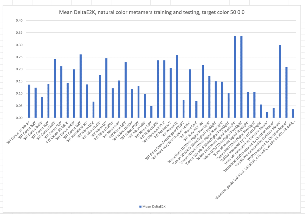
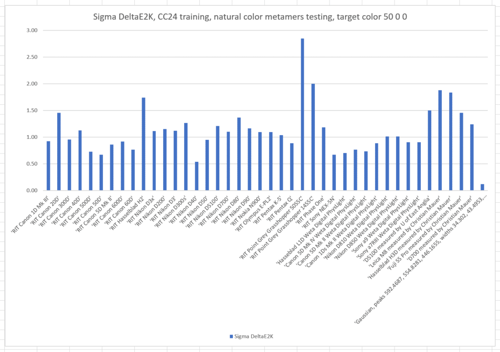
Here’s the results of a run with the metamer color L* = 50, a* = 0, and b* = 0, with the cameras all trained on those metamers:

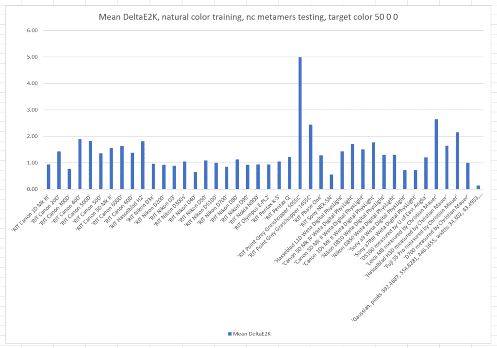
The names of the cameras are across the bottom of the graph. The vertical axis is the mean color error in CIE DeltaE 2000. Take special note of the camera on the far right. It’s not a real camera, but one that I created using optimal Gaussian sensor sensitivity functions(SSFs). In the past, it has produced more accurate results in the simulations than any real camera for which I have the SSFs.

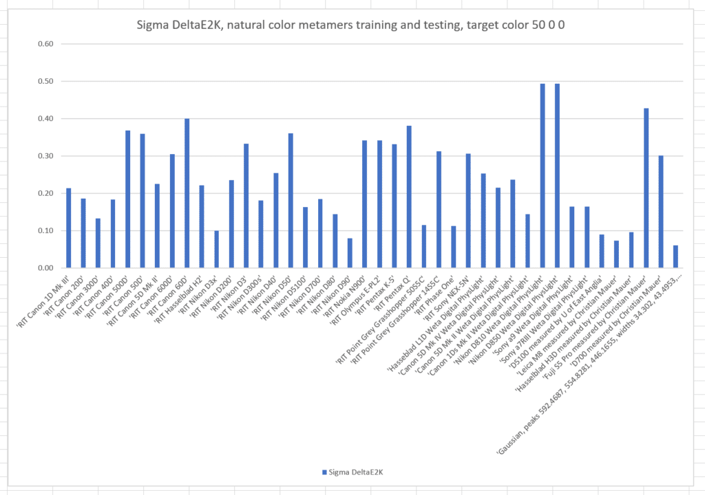
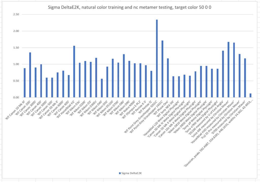
Here are the standard deviations (sigmas) of the colors produced by the cameras:

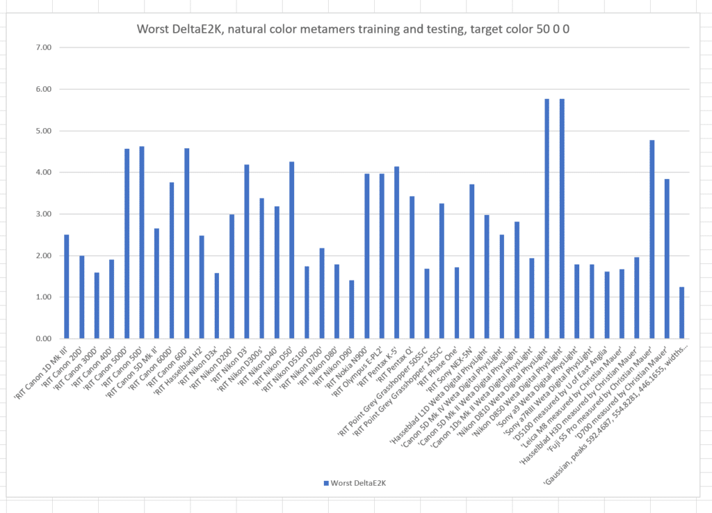
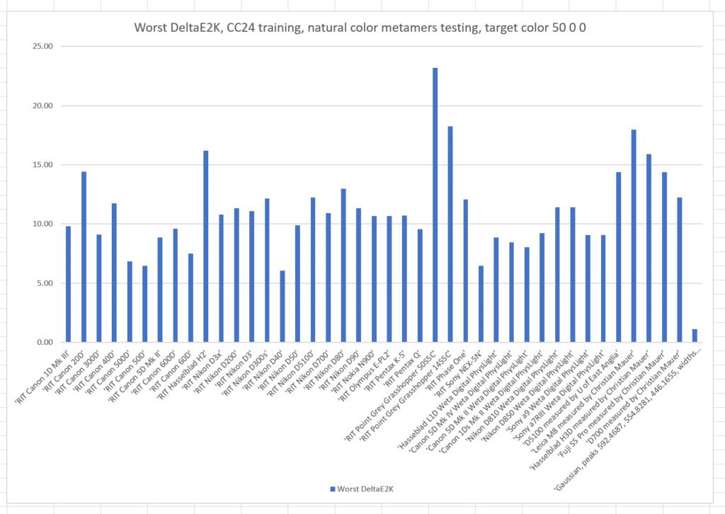
And the worst-case results:

Note by how much the worst results are worse than the standard deviations. This distribution has a long tail.

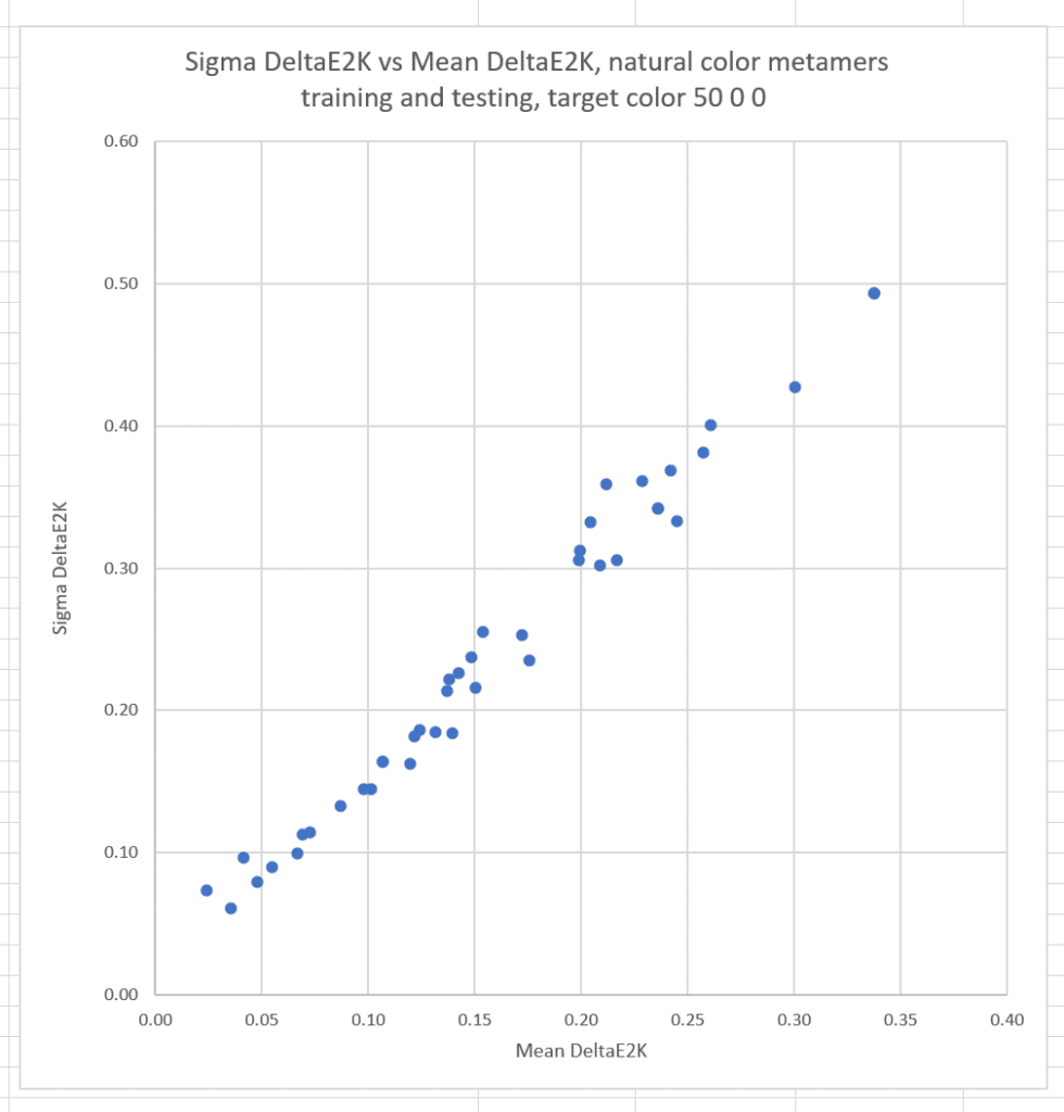
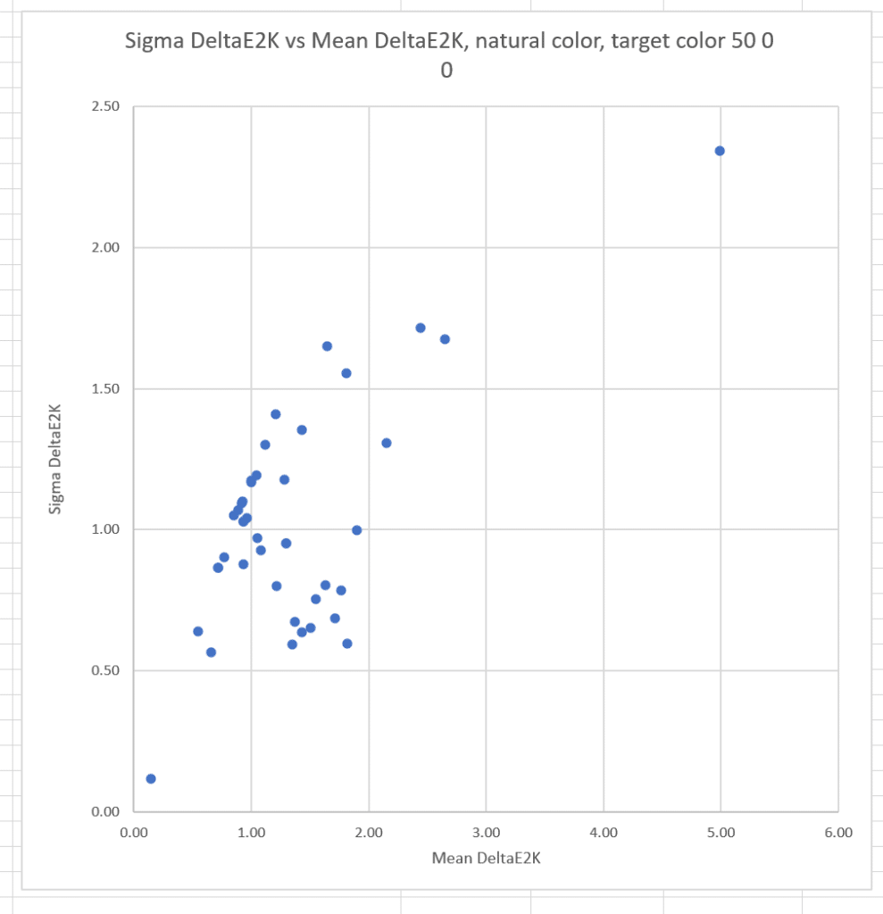
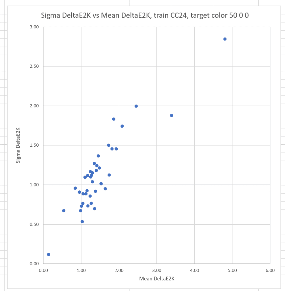
Now I’ll plot the sigmas against the means for all the cameras;

The conclusion is that the more accurate a camera is, the less likely it is to suffer from significant observer metameric error.

That was a pretty restrictive training set. What if we train with the natural colors from which the basis functions were generated, and test with the same metamer set?

The mean errors are much worse. The optimized camera is clearly best.

The sigmas are also much worse. The optimized camera is clearly best.

The worst case errors are also worse. The optimized camera is clearly best.

The correlation between the mean errors and the sigmas is reduced, but still strong.

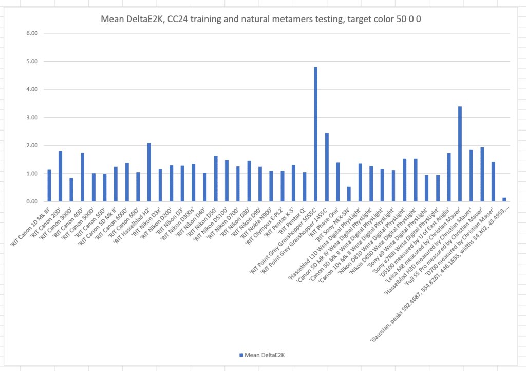
If we train with the Macbetth ColorChecker 24:

The mean errors are somewhat worse than when we trained with the natural color set.

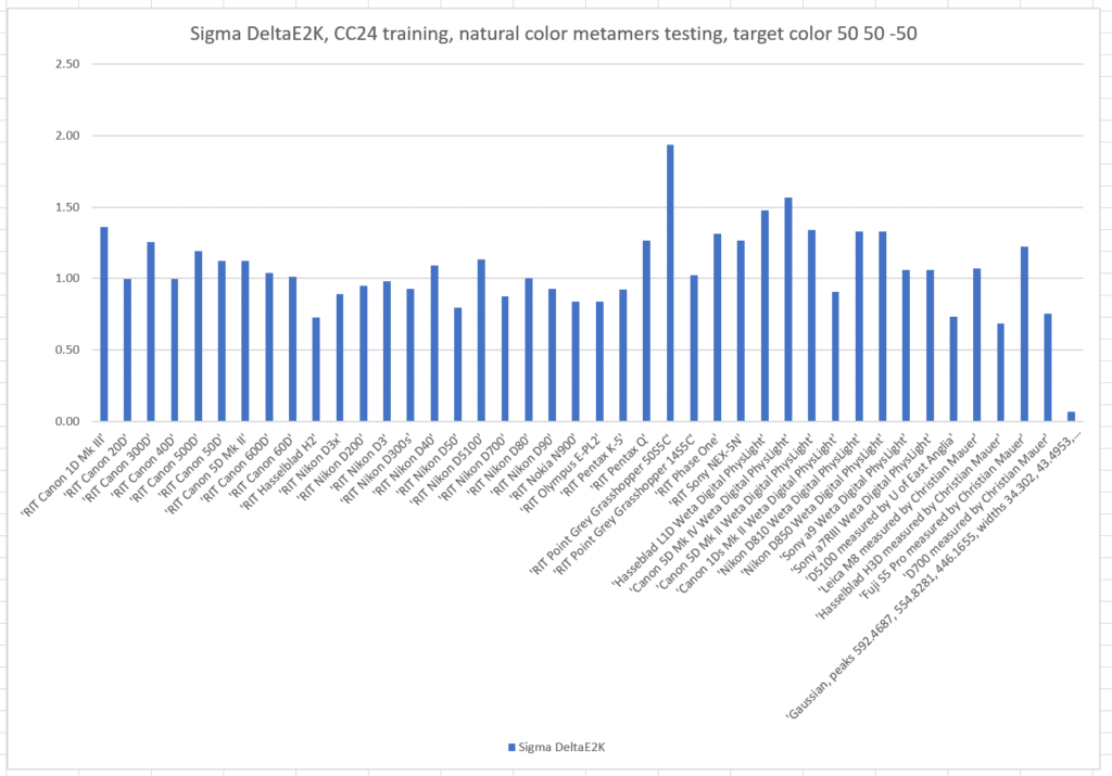
The sigma errors are slightly worse than when we trained with the natural color set.

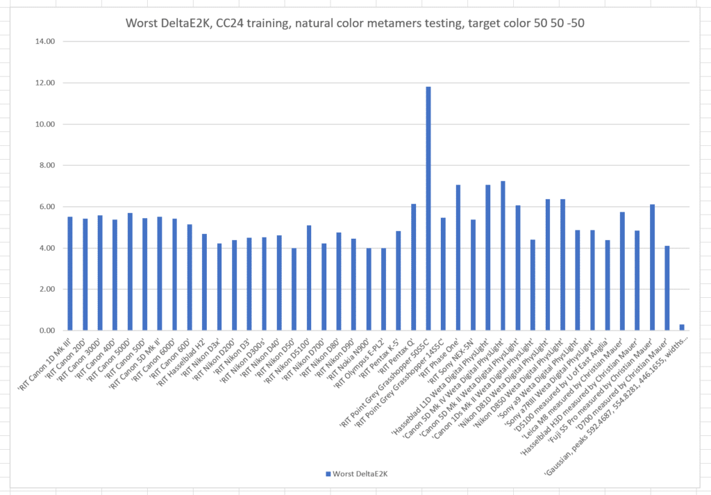
The worst-case errors are slightly worse than when we trained with the natural color set.

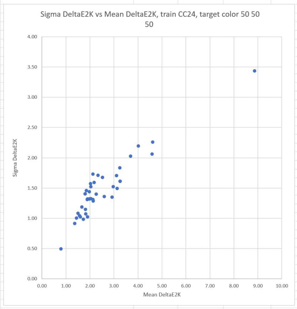
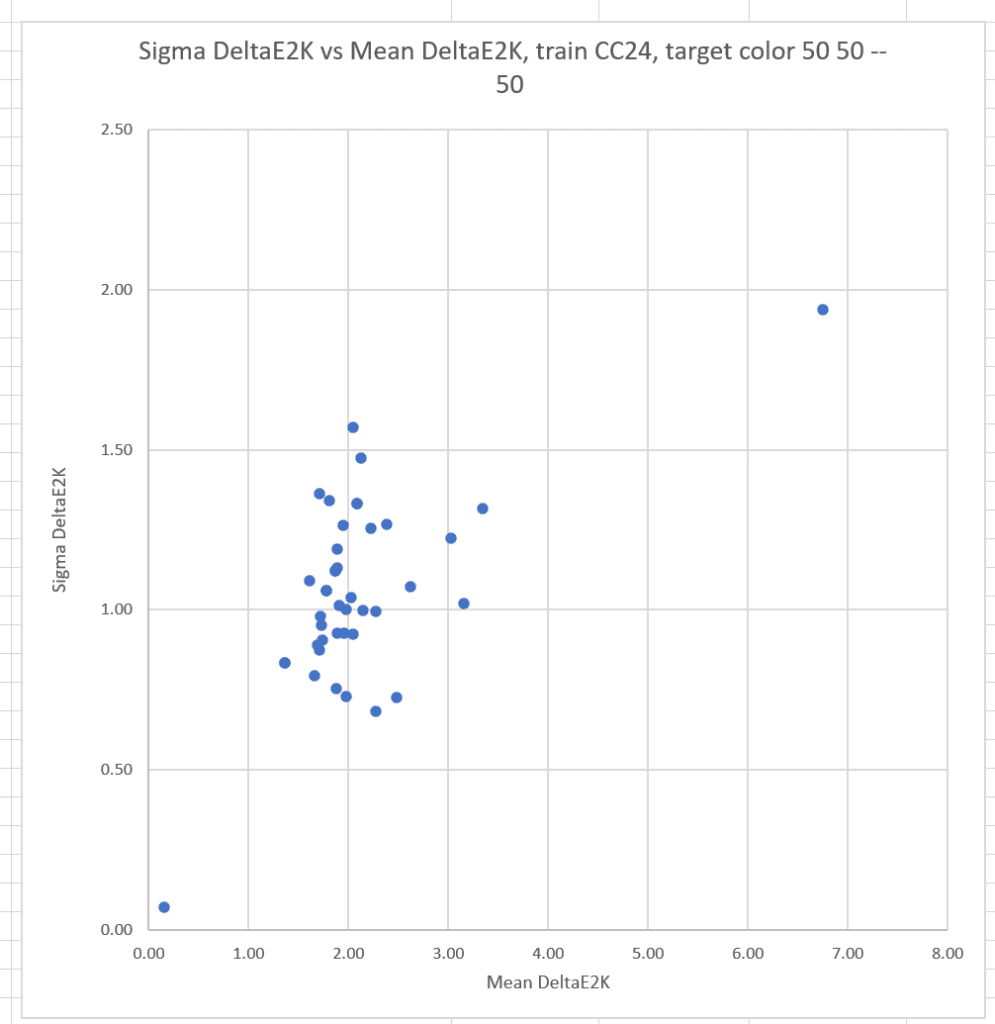
There is still a strong correlation between the means and sigmas.

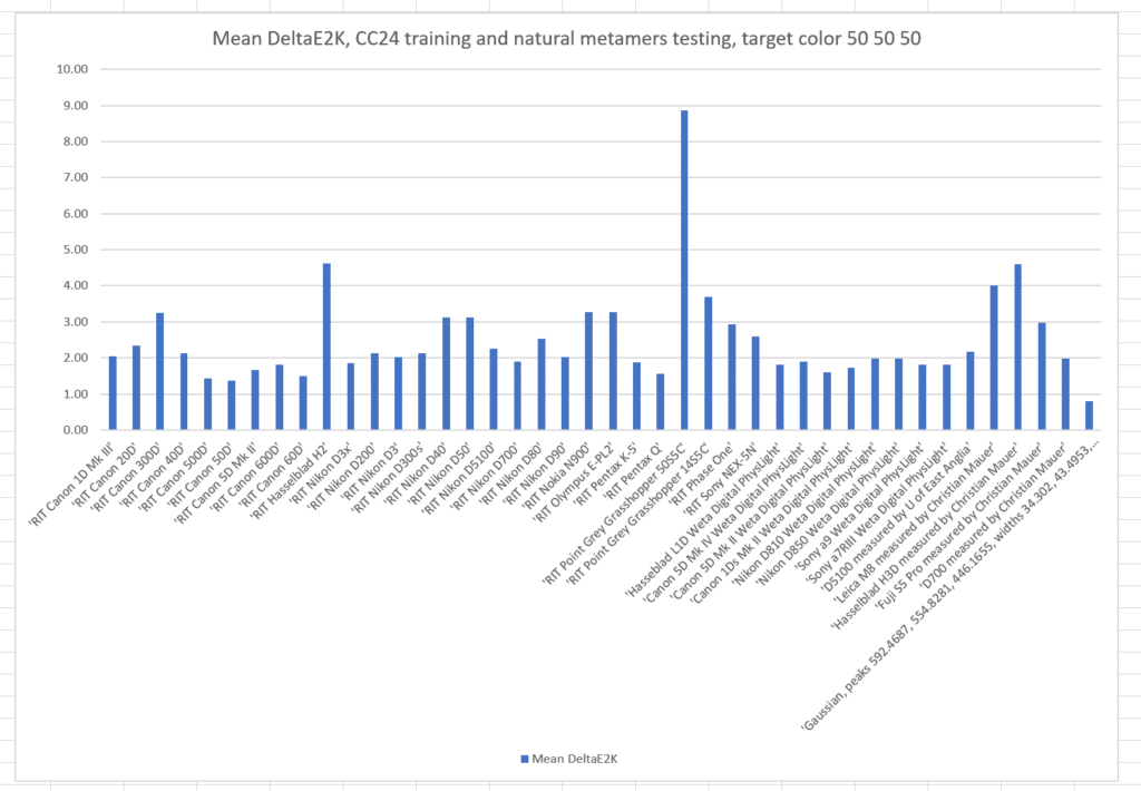
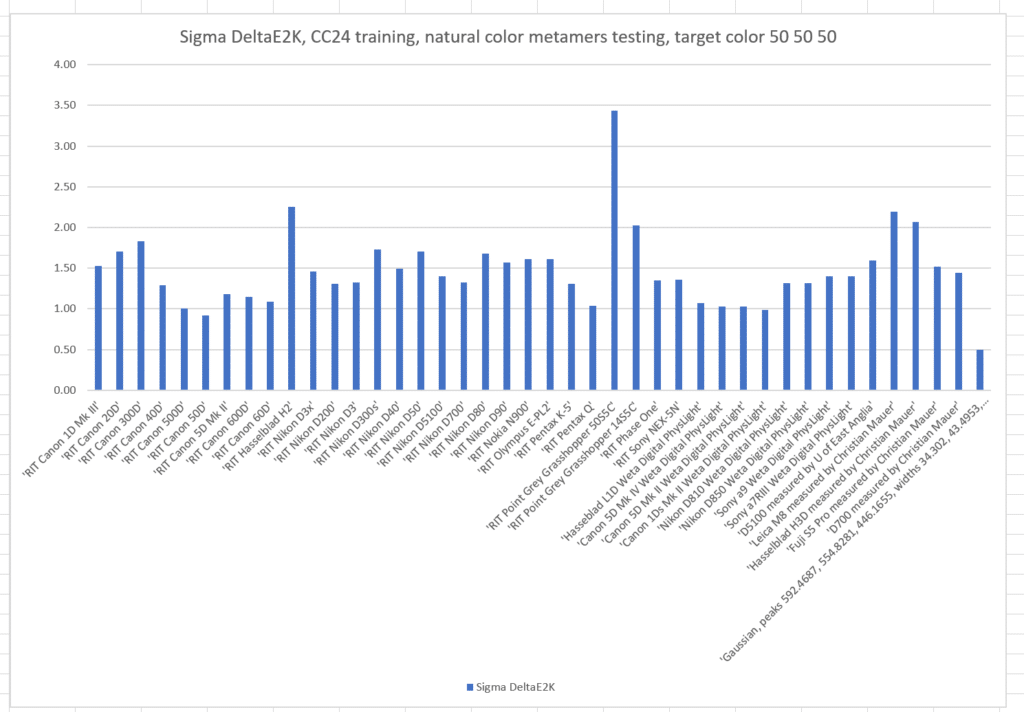
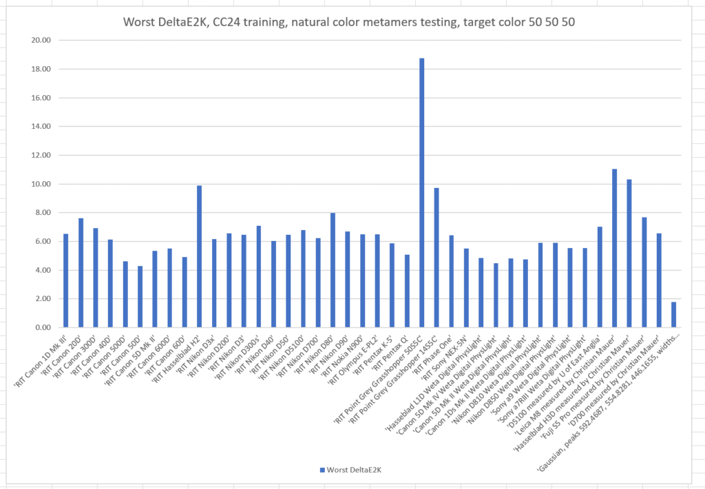
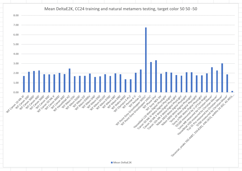
What if we pick another target color, this time L* = 50, a* = 50, and b* = 50? This is a quite-chromatic red.

Here are the same graphs for L* = 50, a* = 50, and b* = -50:

I’ll be doing some more work with this, but my initial, tentative conclusions are:

More accurate cameras produce less observer metameric error than less accurate ones. (That’s not a surprise)

Training on something close to the testing set helps both mean errors and observer metameric error. (Also not a surprise)

Training on the CC24 isn’t all that much worse than training on the set from which the basis functions were generated. (That is somewhat of a surprise)