This is the fourth post on balancing real and fake detail in digital images. The series starts here.
A reader asked me to look into the effects of optical low-pass filters (OLPFs) on sub-Nyquist sharpness and aliasing. It was an interesting exercise for me, and I hope you’ll be interested in the results. Such filters used to be common on the highest-resolution cameras, but they have fallen out of fashion as the resolution of cameras has increased. The feeling among manufacturers and users seems to be that for cameras with more that 24 megapixels, lens aberrations, defocusing, and diffraction will reduce aliasing to a tolerable level. Leica even leaves off the anti-aliasing (AA) filter on their 24 megapixel M-series cameras. Nikon used to have a 36-megapixel camera with an AA filter, but they no longer make the D800.
Is this abandonment of anti-aliasing filters a good thing? From my experiences (especially comparing the GFX 50S and GFX 100), I think the opposite, but it’s a good idea to look at what’s happening in detail, and I intend to do that in this post.
At this point, it would be a good idea to give you all a refresher on how OLPFs work. Jack Hogan has already written an excellent treatise on that, and I recommend that you at least skim it before proceeding.
OK, you’re back. I’m going to build on what Jack wrote, with illustrations from some computer modeling of lenses and cameras that I’ve been doing recently. I am indebted to Jack for some of the Matlab code that I’m using, and Brandon Dube helped Jack with parts of that.
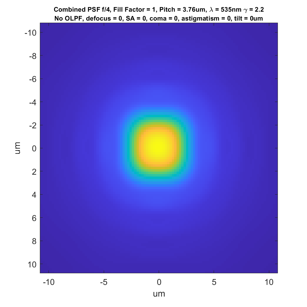
I’m going to start out by showing you something with which you’re probably familiar, a diffraction “haystack”. However, you may not be used to looking at it in this way. This is the point spread function of an ideal f/4 lens in 535 nm monochromatic light (this is about the tightest point spread function that a real-world lens is likely to lay down on a full frame or medium format camera):
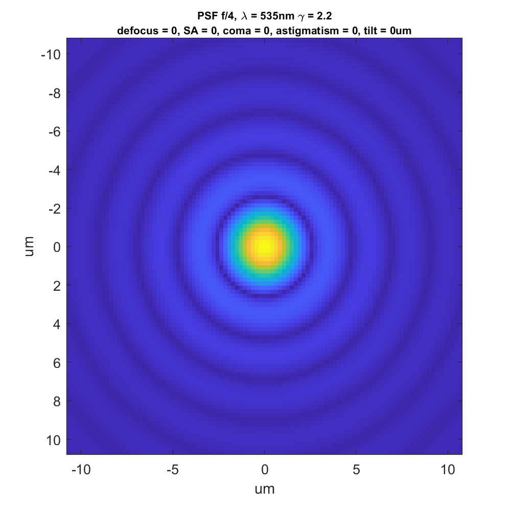
The bright yellow is near 1.0. The dark blue is near 0.0. I added a gamma 2.2 tone curve to the data so that what’s going on in the low parts of the PSF. That’s why the outer rings are so visible.
Now let’s look at something that is virtually identical, but will need a bit of explaining:
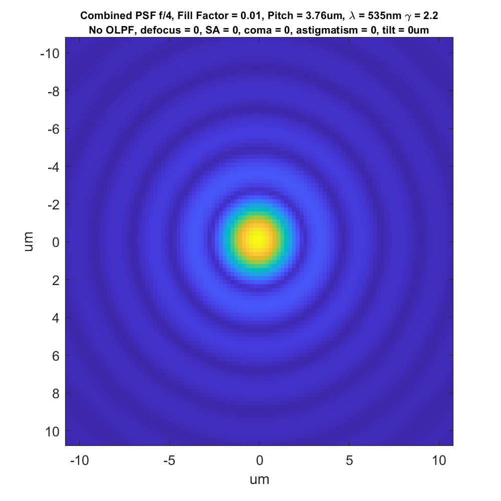
This is the convolution of the PSF in the first image with the pixel aperture of a camera with a 3.76 micrometer (um) pitch, and a fill factor of 1%, making it close to a point sampler. I call this the combined spread function (CSF). We can calculate the modulation transfer function (MTF) of the camera/lens combination from this data; we’ll get to MTFs further on down the page.
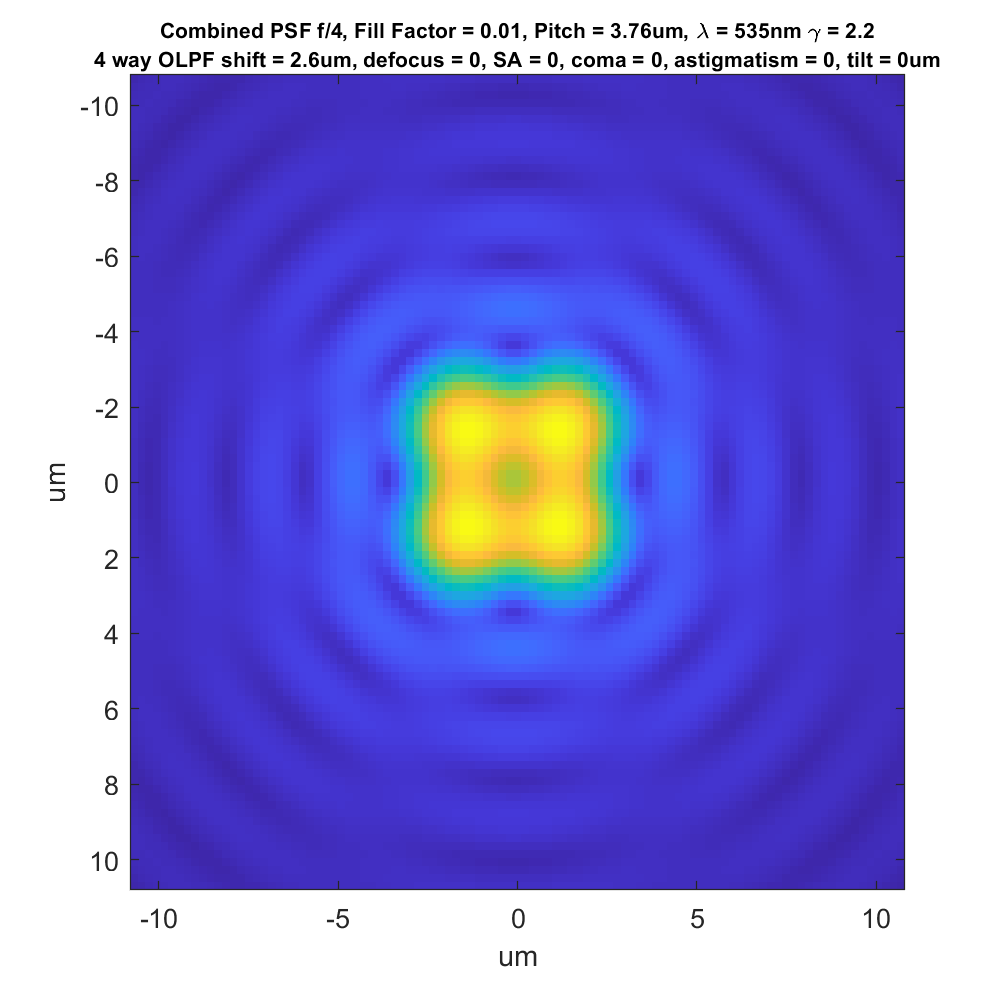
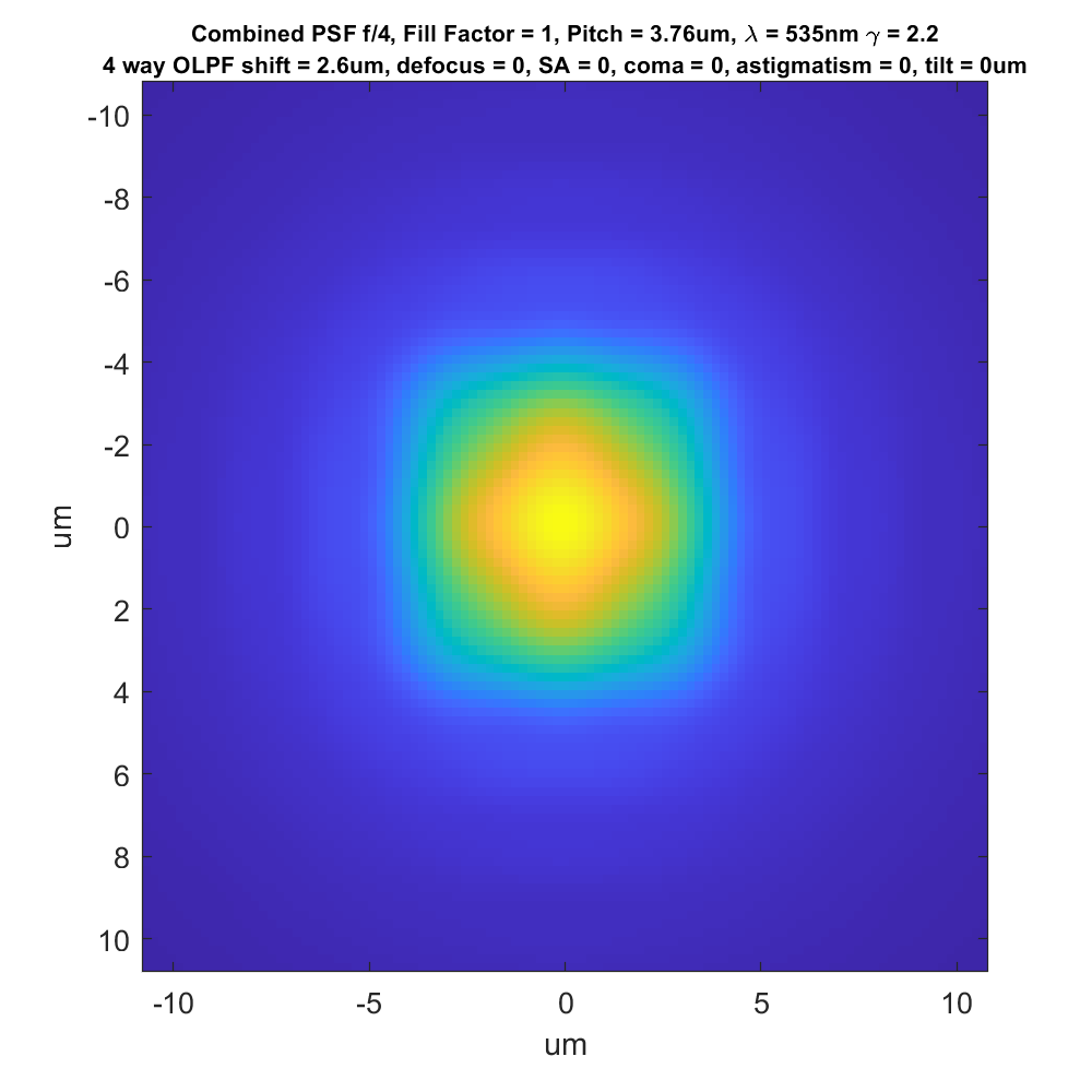
Now let’s add a 4-way (or 4-dot, in Jack’s terminology) OLPF:
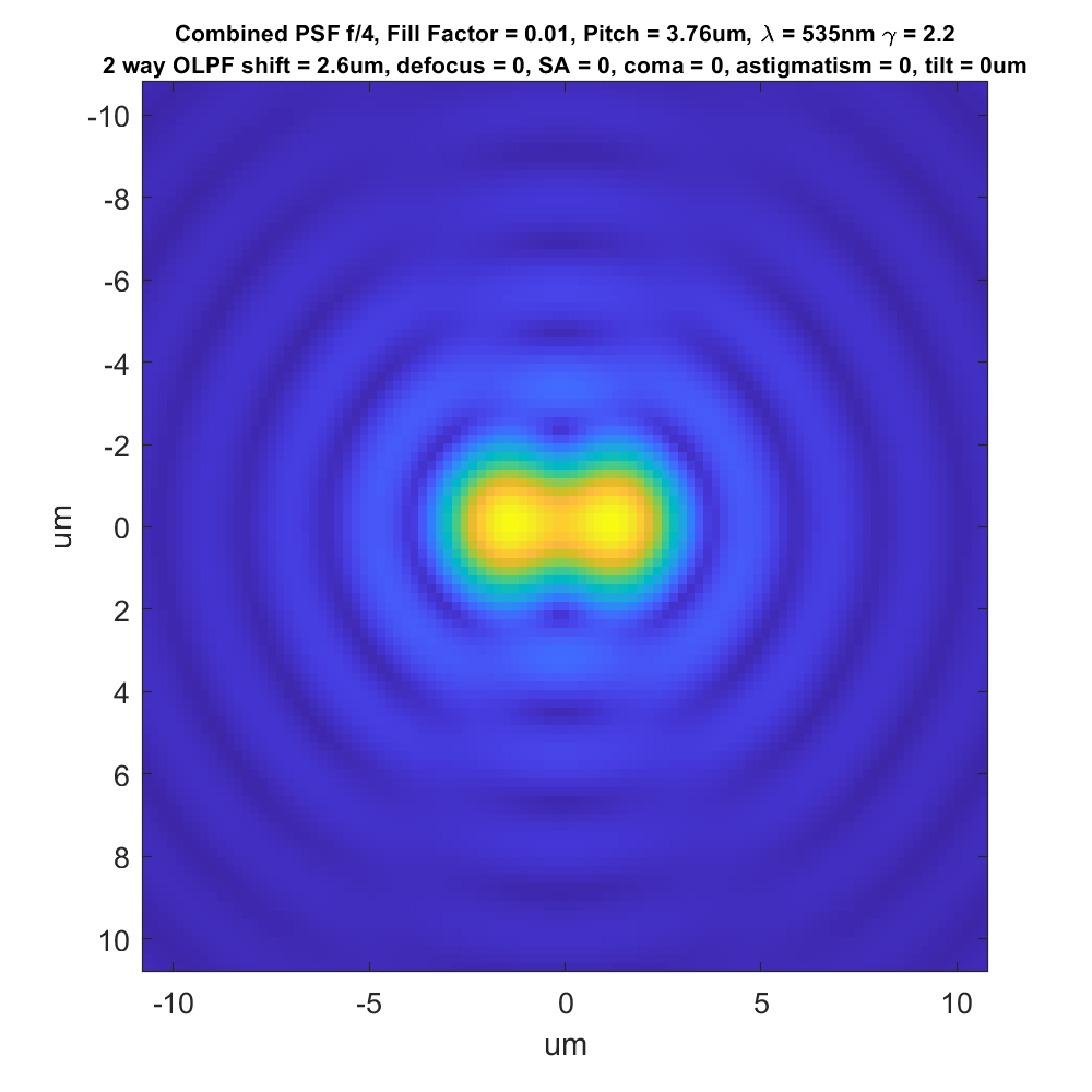
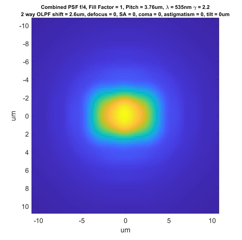
Some cameras use 2-way OLPFs. Here’s what the combined point spread function looks like for a camera like that above that just shifts horizontally:
Here’s the CSF for a camera with no OLPF with a fill factor of 100%:
The sensor is now introducing quite a bit of blur relative to the diffraction solid. Now let’s see what happens to the CSF for our 4-way-OLPF-camera with the same fill factor:
The camera sensor’s blurring has forced the four peaks to become one. That’s a good thing. It’s also made the overall curve a bit broader. Is that good or bad? We’ll have to see when we start looking at MTFs.
For completeness, here’s the 2-way OLPF with 100% fill factor:
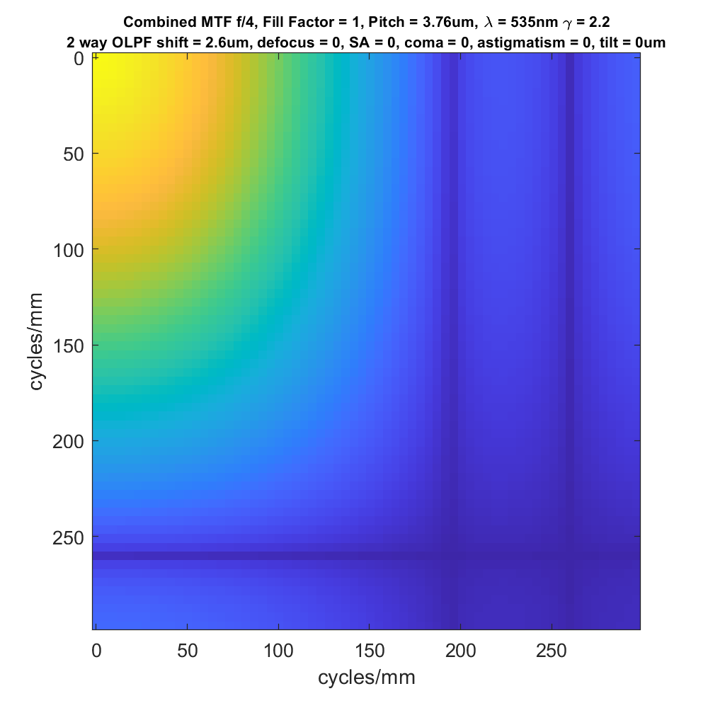
If we look at the two-dimensional modulation transfer function for the 4-way case, we get this:
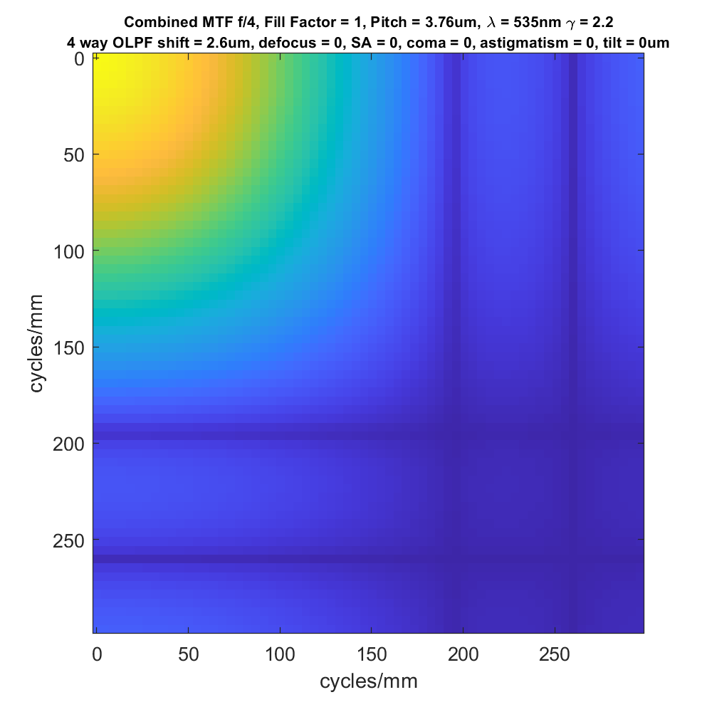
There are two sets of zeros in both the horizontal and vertical directions. The first set (the one closest to the origin at the top-left of the graph) is caused by the OLPF and occurs about 0.7 cycles/pixel. The second set is caused by the pixel aperture, and occurs at about 1 cycle/pixel.
Looking at the 2-way case:
We see that in the vertical direction, the sensor behaves about as it would were there no AA filter.
I want to show you some one-dimensional MTF curves, so I’m going to drop the 2-way OLPF case for the rest of the post. Continuing with it would require too many graphs.
Here’s the one-dimensional MTF curve for the 4-way OLPF camera above:
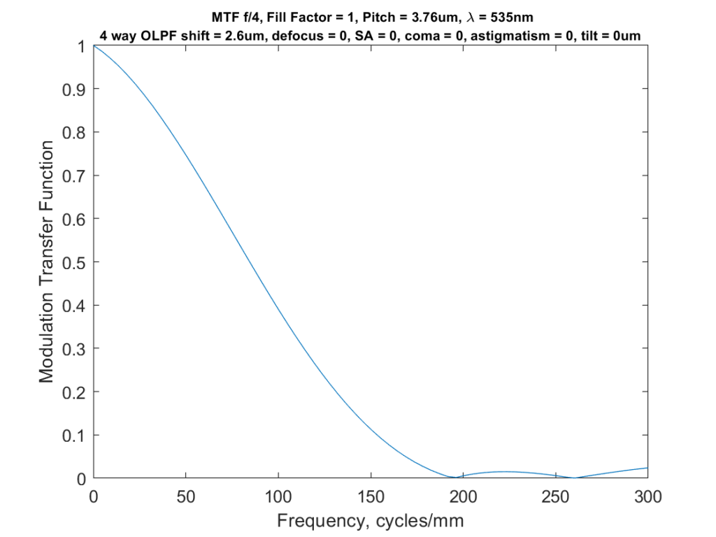
Now you can see how little energy there is about about 200 cycles per millimeter.
Since we’re concerned with aliasing, we can change the horizontal axis to cycles per pixel:
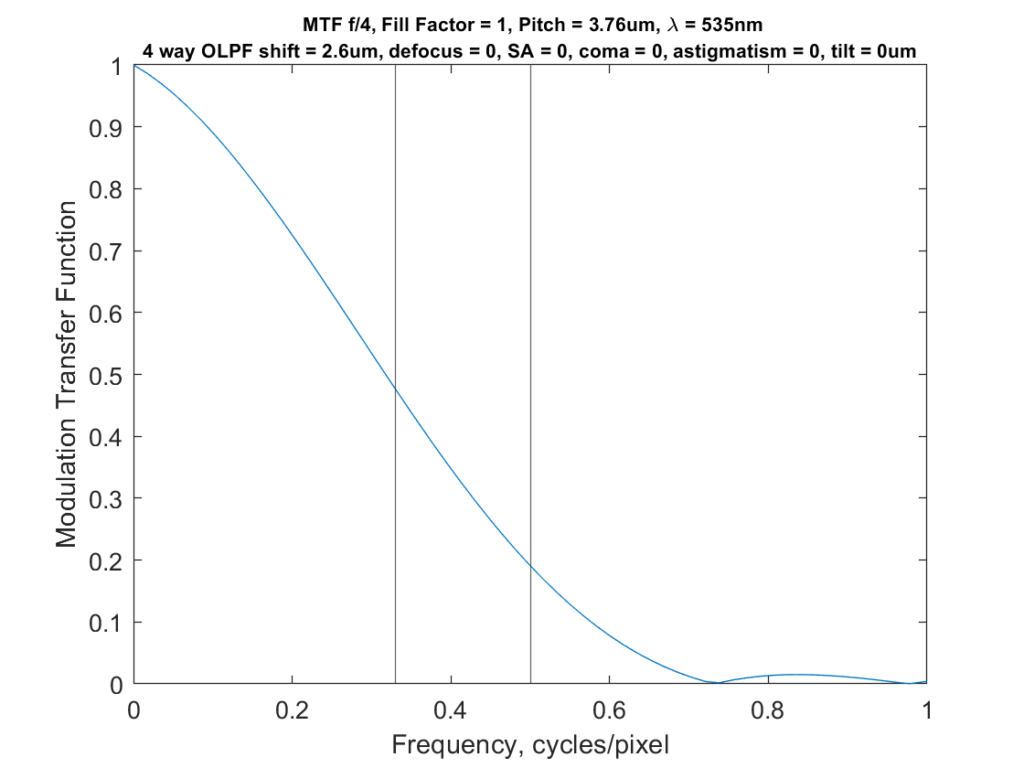
I’ve plotted vertical lines at the Nyquist frequency (half a cycle per pixel) and what I consider to be a useful approximation of the Nyquist frequency for sensors with a Bayer color filter array (a third of a cycle per pixel).
Now let’s look at the MTF energy below the Nyquist frequency vs that above it as a function of f-stop, with and without the OLPF:
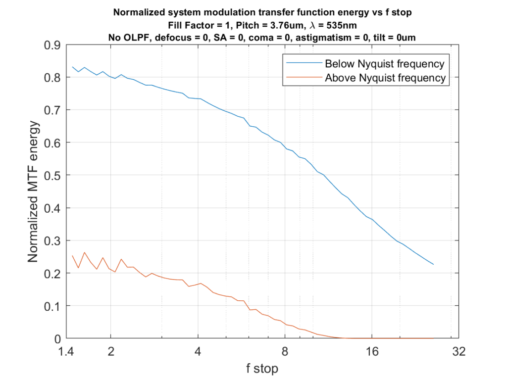
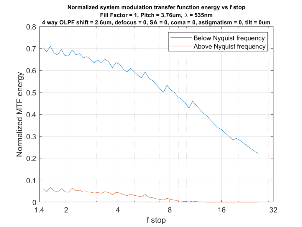
There is a substantial amount of reduction in above-Nyquist-frequency energy in the lower graph, and a small penalty in below-Nyquist energy.
If we consider 0.33 cycles per pixel to be the effective Nyquist frequency for a Bayer-CFA sensor, we get these curves:
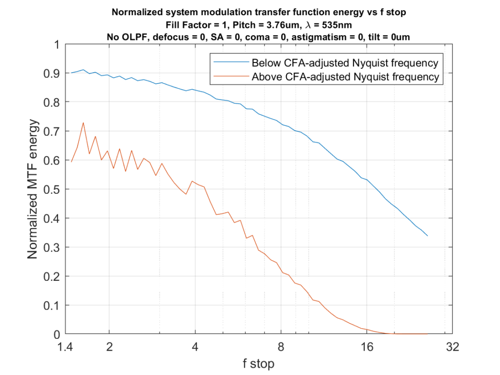
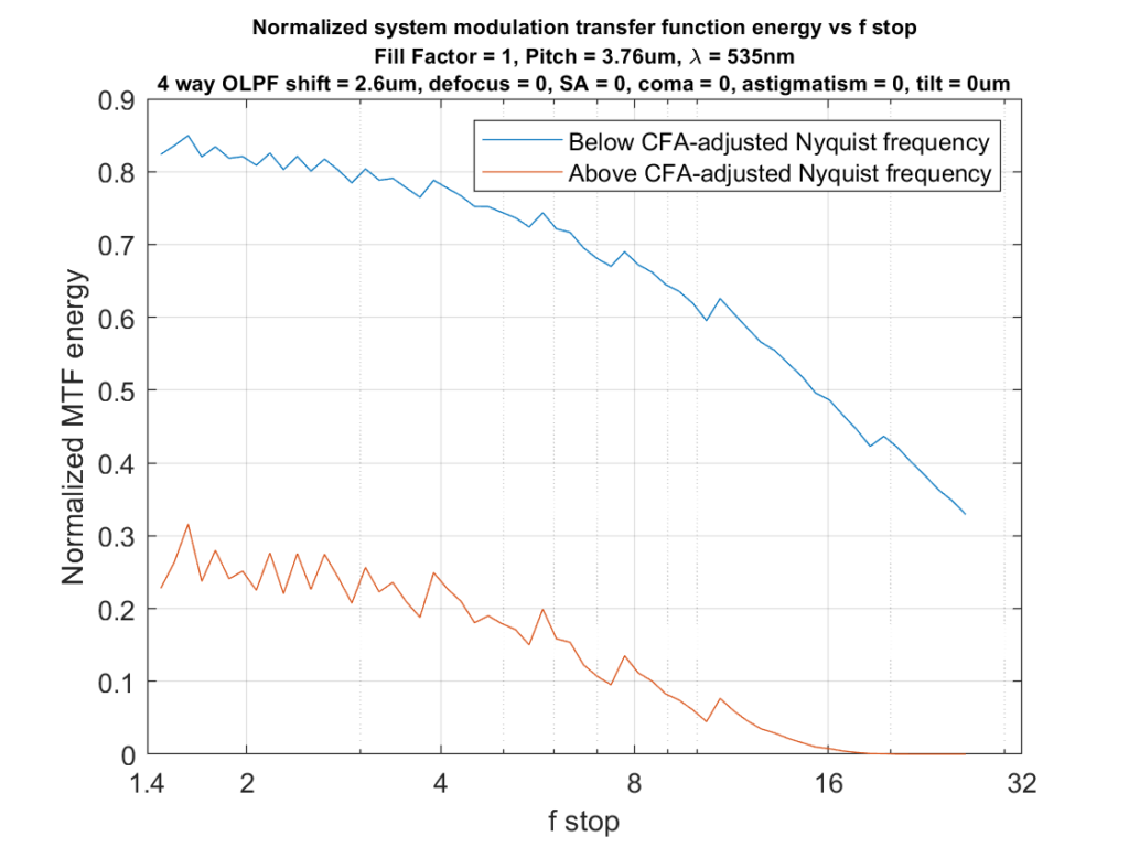
I think you could make an argument that, because of the effects of the CFA, the 0.7-times-the-pitch OLPF offset is too low. I think it’s hard to make an argument that we’d be better off without it, if avoidance of artifacts is important.
All the above assumes a truly excellent lens. I can, and will, if asked, demonstrate what happens when the lens has aberrations. But let me point out that the worse the lens is, the less the relative effects of the OLPF, so adding lens aberrations isn’t going to make the filter-less sensors look better in these metrics, it will just make the two cases look more the same, as does diffraction on the right-hand side of the above curves.
Fair warning, W020 (defocus) and W040 (third order spherical) are woefully not enough to cover the aberrations of any lens faster than, say, F/4, or designed after, say, 1960.
Thanks. I’ve got more thanks to your Matlab code, but the dimensionality of the space thus defined is daunting. Of course, all those were zeroed out for the simulation in this post.
If you limit to on-axis study, it isn’t so bad. You just (absolutely) need the next radial order, W060. You probably can round off W080, and certainly can round off everything higher than that. But the chromatic aberrations (axial color, dW020/dlambda) and spherochromatism (d[W040, W060, …]/dlambda) are not ignore-able. And when you do polychromatic propagations, you need to take special care to match all the samplings in the PSF plane.
Axial color is well approximated by a low order polynomial, either quadratic or cubic with points of equal focus around blueish (say, 480 nm) and redish (say, 580 nm). Non-apo lenses will be quadratic, and apos cubic or possibly (unlikely) higher order.
I have never looked at what polynomial spherochromatism is, if it is one at all.
Coma, astigmatism, etc, can be disregarded on-axis (they should be zero).
I have some code lying around you could convert from numpy to matlab (not hard, it’s a short function) that uses the matrix triple product Fourier transform for a fast transform onto a grid of arbitrary sampling; you just sub out the i/fftshift and fft2 with mfft2, then the arrays have slightly different Q (no issue if > 2) but the same sampling, so you can just stack and average or spectrally weight.
Looking at the curves, I would think that monochrome aliasing would be negligible beyond f/8 even without the OLP filter.
With the CFA it seems that f/16 may be needed for unalised imaging.
Obviusly, an OLP filter may help a lot, and my guess is that the loss of MTF by the OLP filter would be easily compensated by sharpening.
Some food for thought.