Presenting capture accuracy results: the basics

This is the fourteenth in a series of posts on color reproduction. The series starts here.

I am writing Matlab code to automate the crunching and presentation of camera captures of Macbeth color checker charts. The purpose is to provide a way to test capture and raw developer accuracy. I’ve written code that does the basic analysis, I’m working on how to present the data. Today, I’ll show you what I’ve done so far.

The camera and the raw developer that I used to get the data shown here don’t matter in this context, so I’m not going to address that issue,

First, a plot of the CIELab Delta-E for each patch:

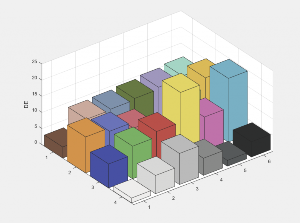
I’ve shaded the columns so that they’re about the same color as the patches. Like that?

Now, a look at just the chromaticity errors, also in Lab:

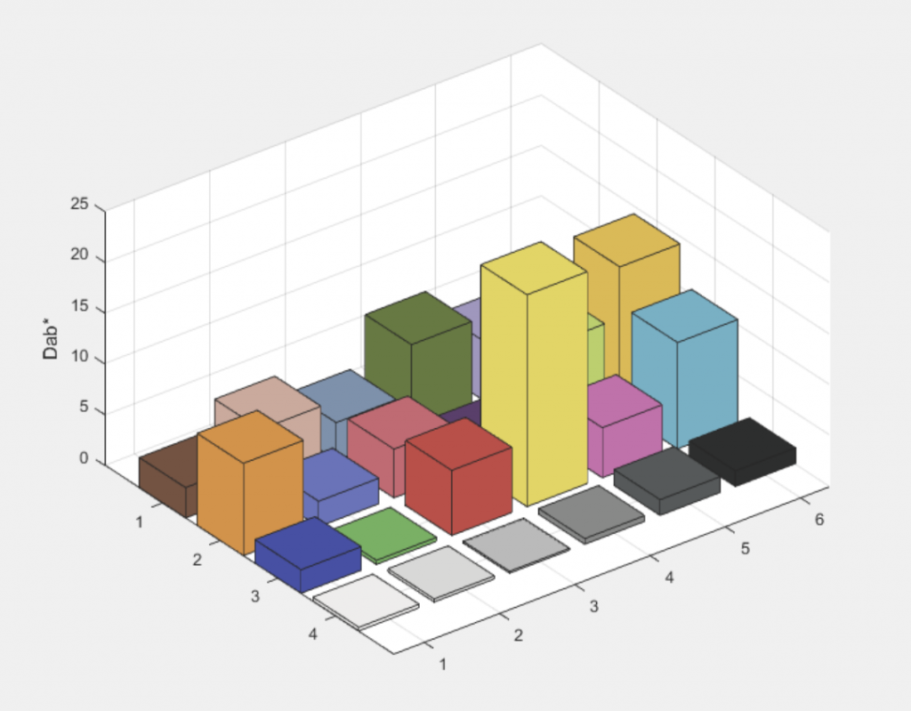
Hmm. The upper right corner is obscured by the two yellowish patches. In Matlab, you can rotate the graph to see what’s going on there, but I can’t post the interactive graphs on the web. I think varying the viewing angle with each graph would be confusing.

Now, a look at the chromaticity errors in more detail in Lab:

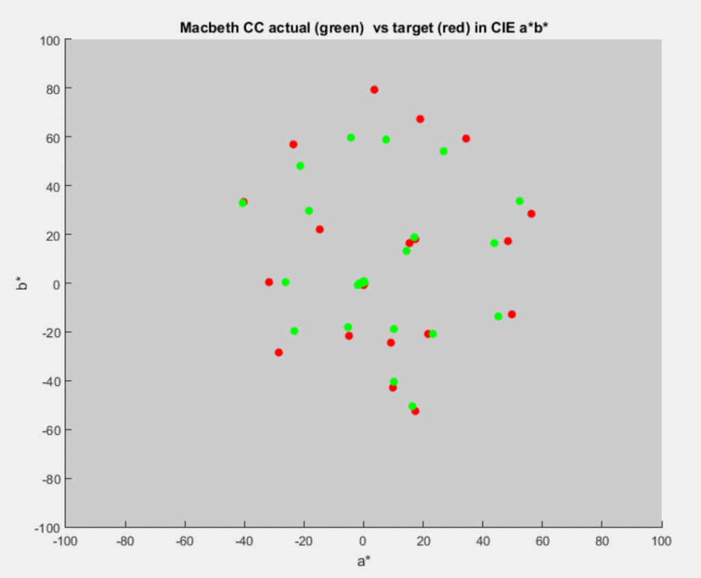
I’ve pinned the axis range to [-100, 100] for both axes. That means that plots are easy to compare, but reduces the magnification from what would be available if I fitted the ranges tightly for each plot.

Here’s the same data in Luv:

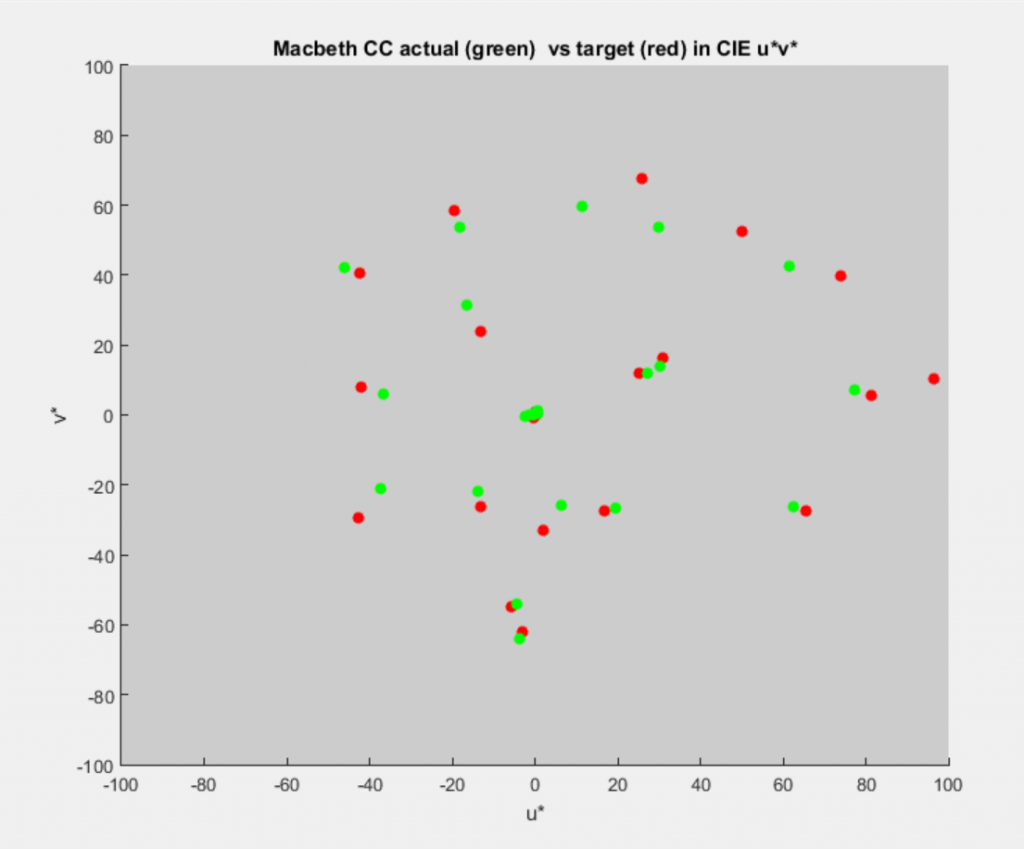
Whether you like Lab or Luv for this probably depends on your level of familiarity with each. I’ll probably use Lab mostly, since photographers tend to be more comfortable with it.

I will also be looking for some overall scalars that represent important qualities, such as color twist. Those will be useful for comparing sets of captures or developments with different cameras, processors, or lighting.

Comments are welcome.