This is one in a series of posts on the Fujifilm GFX 100. You should be able to find all the posts about that camera in the Category List on the right sidebar, below the Articles widget. There’s a drop-down menu there that you can use to get to all the posts in this series; just look for “GFX 100”. Since it’s more about the lenses than the camera, I’m also tagging it with the other Fuji GFX tags.
In the previous post, I looked at the microcontrast of the Fujifilm 120 mm f/4 GF lens at minimum focusing distance (MFD) with and without two 18mm extension tubes. In this post I’m going to look at lens sharpness versus focal plane displacement for each of the raw color planes.
Here’s a picture of the setup:
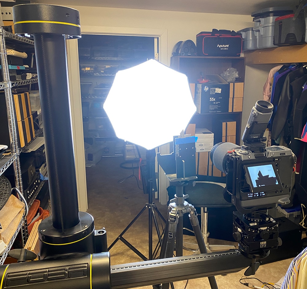
Here’s the test protocol:
- GFX 100
- Foba camera stand
- C1 head
- 2 each 18mm Fuji extension tubes
- Lens focused to close to as near as it would focus
- ISO 100
- Electronic shutter
- 10-second self timer
- f/4 through f/11 in whole-stop steps
- Exposure time set by camera in A mode
- Focus bracketing, step size 1, 150 exposures
- Initial focus short of target
- Convert RAF to DNG using Adobe DNG Converter
- Extract raw mosaics with dcraw
- Extract slanted edge for each raw plane in a Matlab program the Jack Hogan originally wrote, and that I’ve been modifying for years.
- Analyze the slanted edges and produce MTF curves using MTF Mapper (great program; thanks, Frans)
- Fit curves to the MTF Mapper MTF50 values in Matlab
- Correct for systematic GFX focus bracketing inconsistencies
- Analyze and graph in Matlab
At f/4 in the center, first with the 36 mm worth of extension tubes:
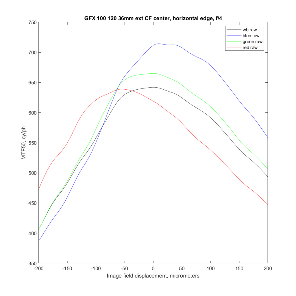
Let me decode the chart. The vertical axis is MTF50 in cycles/picture height. The horizontal axis is displacement of the sensor die (image field) focal plane in micrometers. In the object field (the subject side of the lens) the left side of the chart represents front-focusing, and the right side of the graph represents back focusing. There are four lines plotted. The red on is the red raw channel, the blue one is the blue raw channel, and the green one is the average of the two green raw channels. The black line is a combination of the other three lines after white balancing to the target. It can be considered a stand-in for a luminance MTF50 curve. The white-balanced (WB) raw curve peaks at about the same place as the green curve, since green is the main component of the WB raw curve. However, the peak of the WB raw curve is lower than the green curve, because the red and blue curves don’t peak in the same place as the green curve. That is the result of the lens’ longitudinal chromatic aberration (LoCA).
The height of the black curve at its peak is the best estimate of the sharpness of the lens that can be derived from this chart. In this case, it is a bit lower than the green channel curve because the lens has considerable LoCA.
The same curves with no extension tubes:
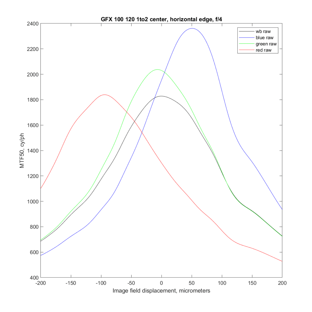
There is a bit more LoCA, but the lens is much sharper here. In fact, if you look at the white-balanced curves, it’s almost three times as sharp!
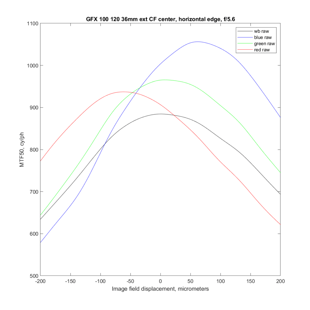
At f/5:6, first with the tubes:
And without:
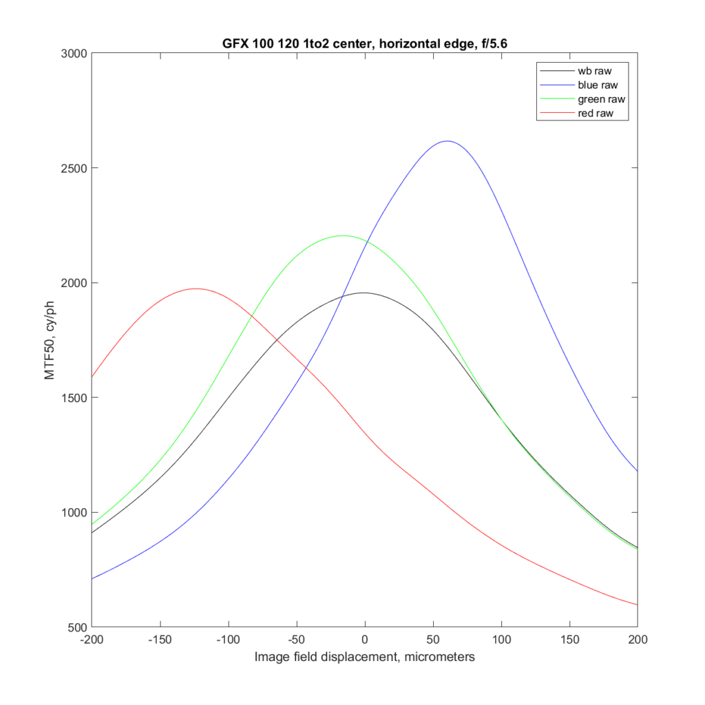
The lens is almost twice as sharp without the tubes.
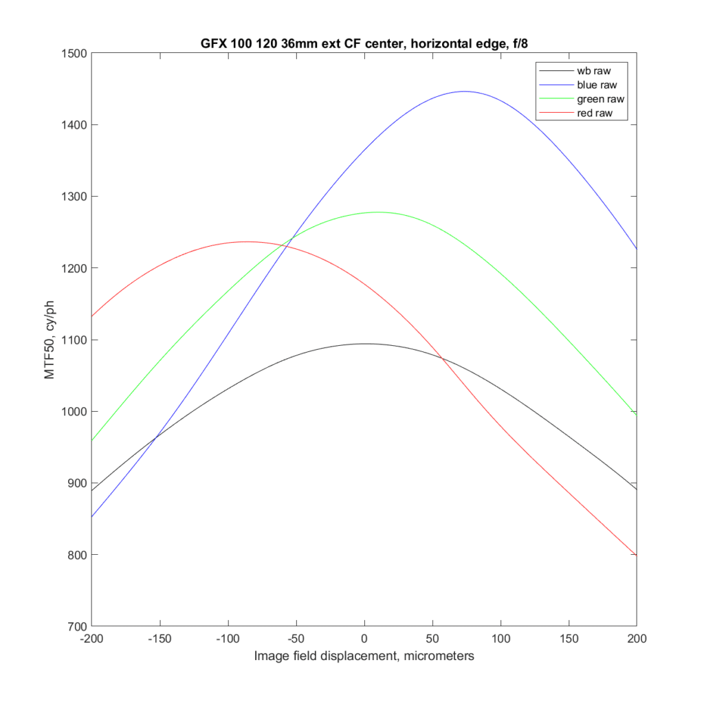
Next up, f/8, first with the tubes:
And without the tubes:
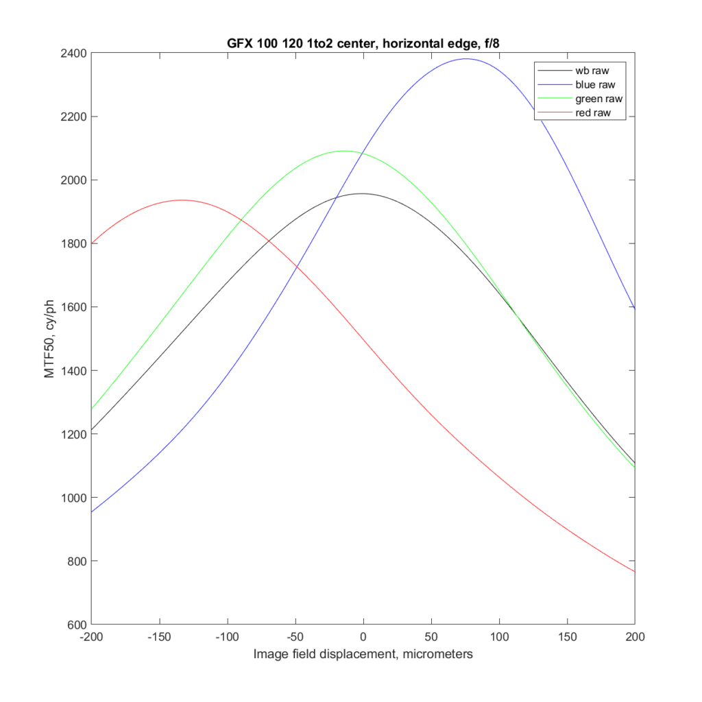
Almost twice as sharp without the tubes.
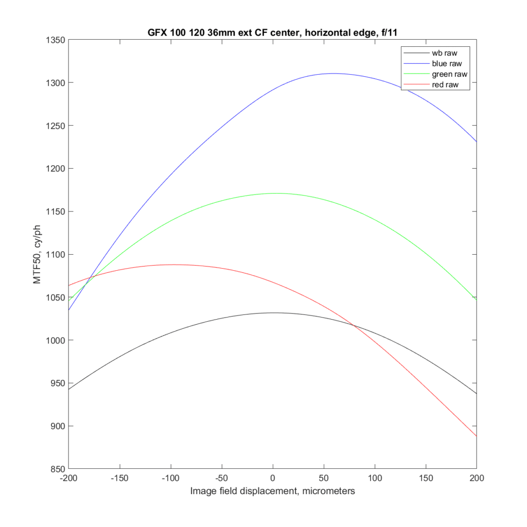
At f/11, with the tubes:
And without:
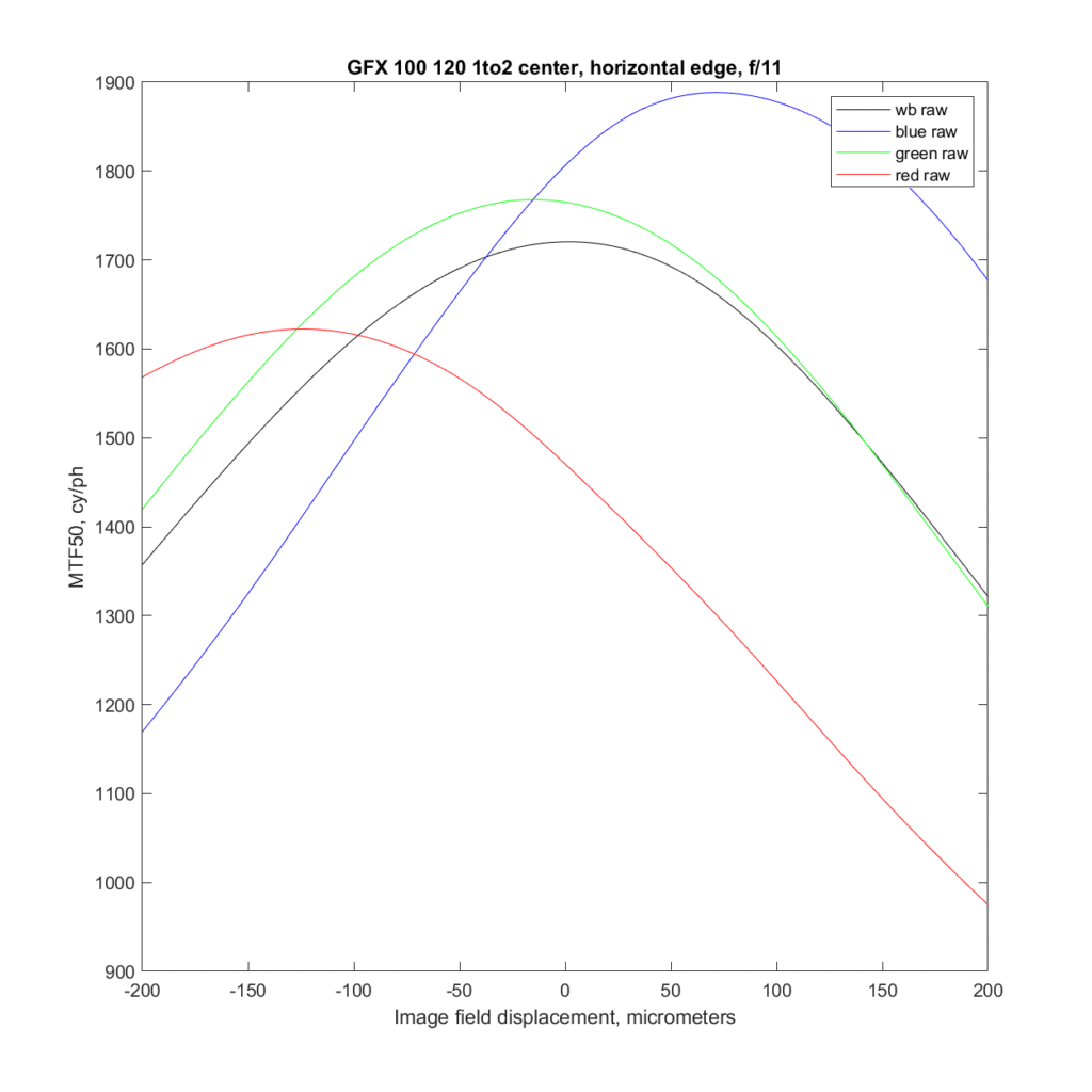
Now, at the far right edge, for a horizontal slanted edge.
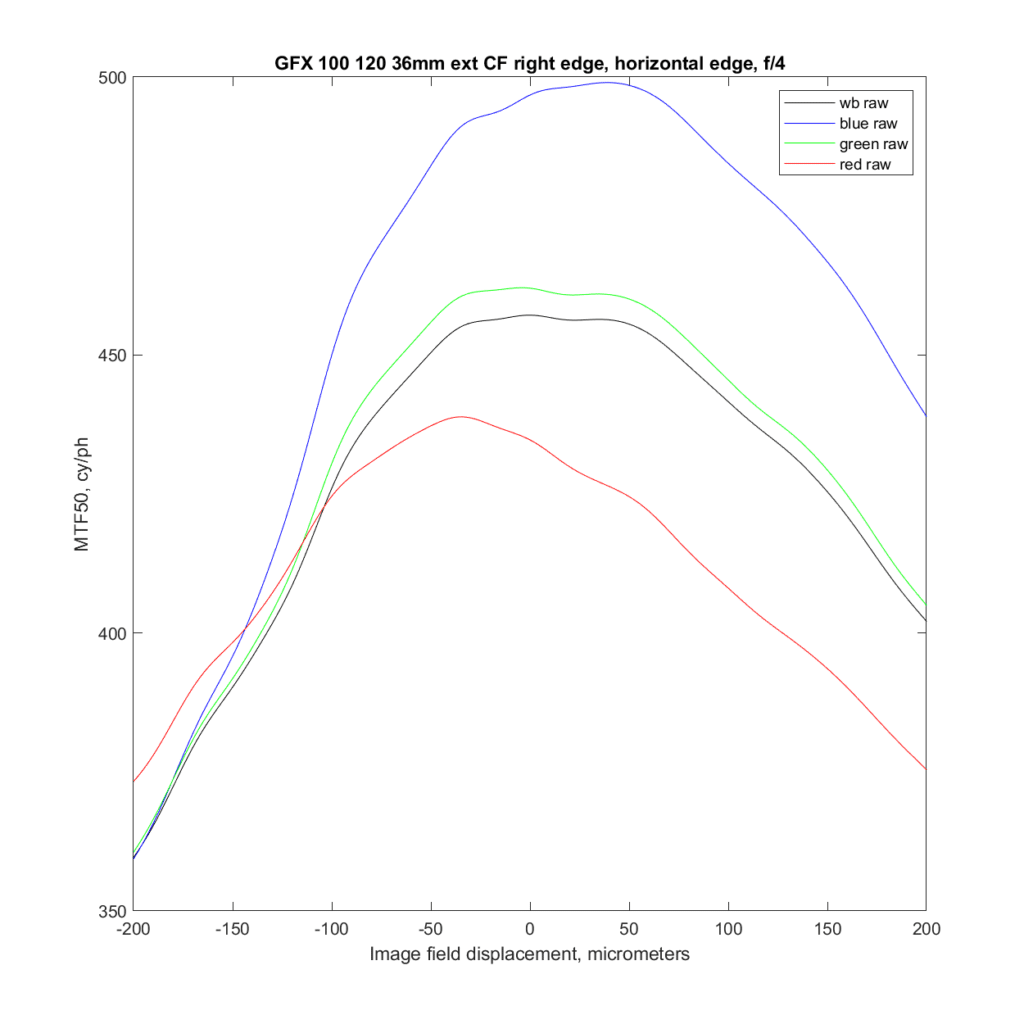
At f/4, with tubes:
And without:
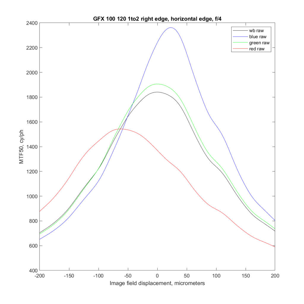
The results without the tubes are more than 4 times sharper.
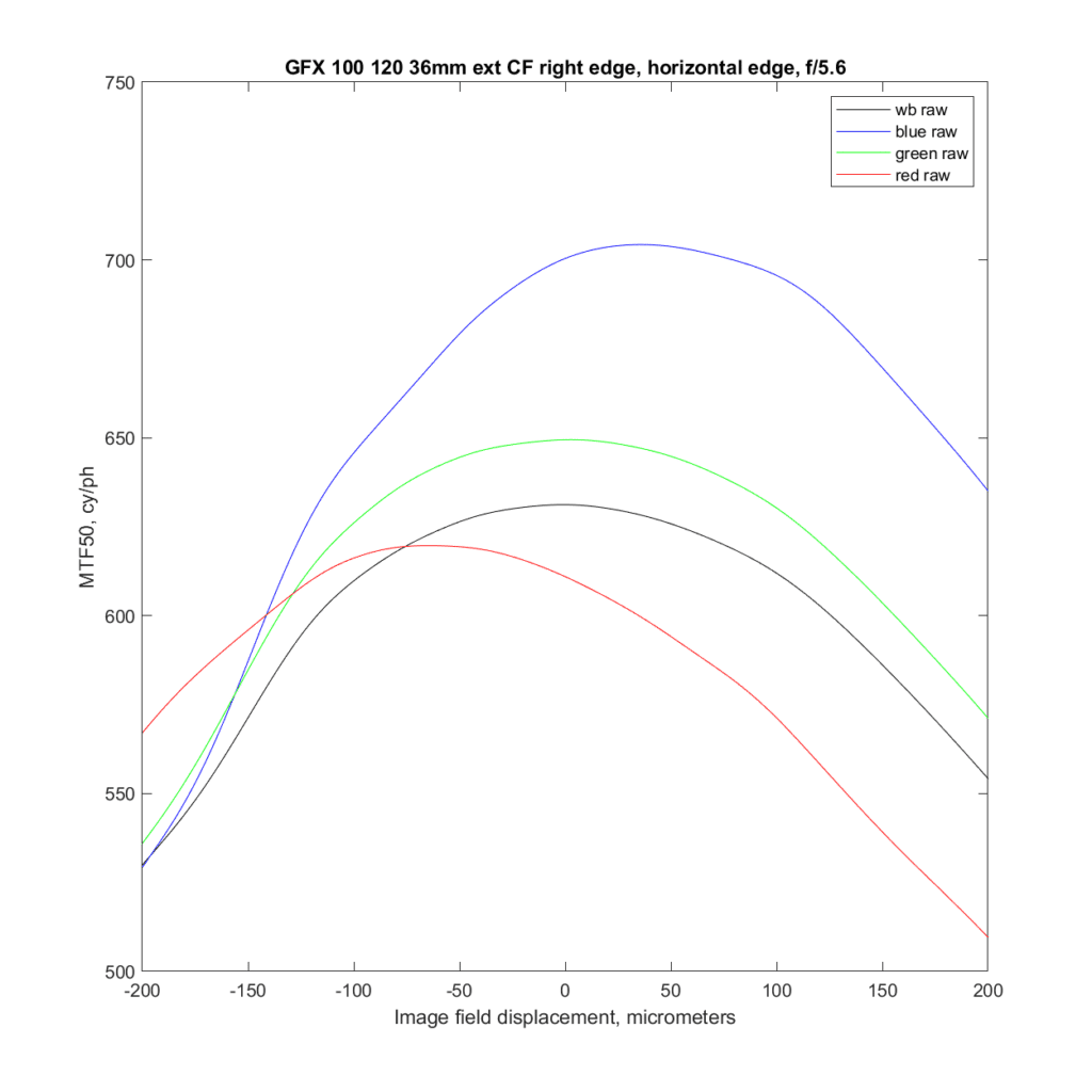
At f/5.6, with tubes:
And without:
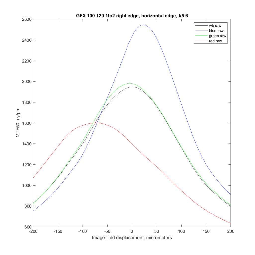
Big difference.
At f/8, with the tubes:
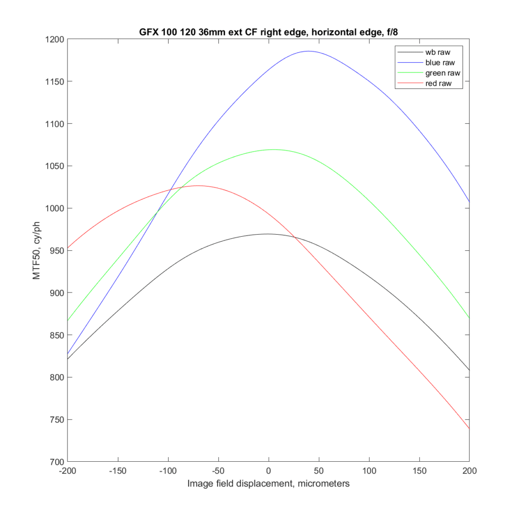 g
g
And without:
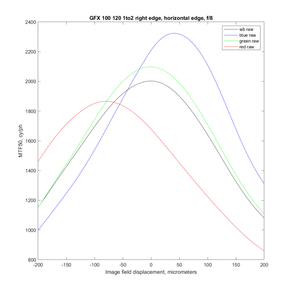
There is still big difference.
At f/11, with tubes:
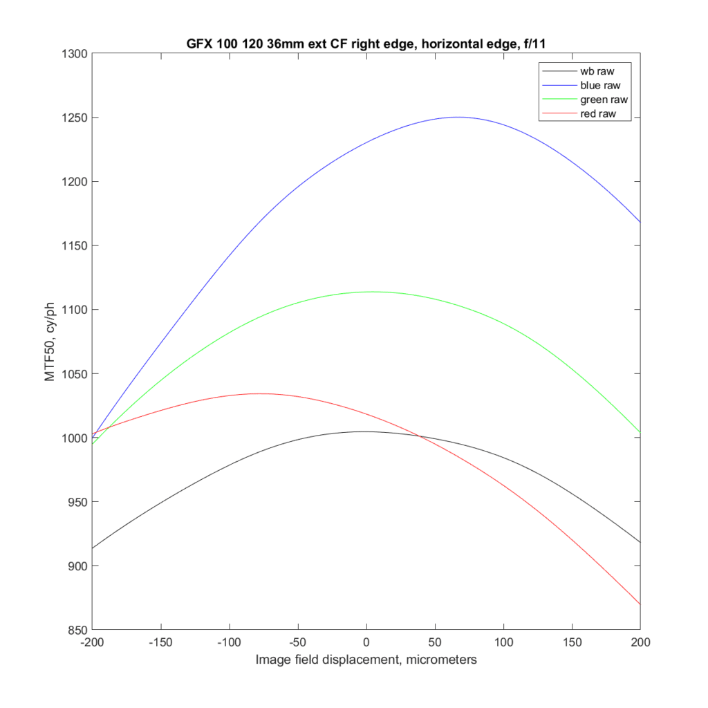
And without:
This test technique calibrates out field curvature. If its effect were included the edge results would look worse, assuming that one focused in the center.
Leave a Reply