the last word

Photography meets digital computer technology. Photography wins -- most of the time.

  • site home
  • blog home
  • galleries
  • contact
  • underwater
  • the bleeding edge
You are here: Home / The Last Word / Luminance and chromaticity vs spatial frequency

Luminance and chromaticity vs spatial frequency

April 20, 2014 JimK Leave a Comment

There was a great thread on the dpreview forum started by Jack Hogan (who has also posted in this blog), about anisotropy in anti-aliasing filters. In the generally erudite and productive discussion that followed, someone (I’d give him credit, but I don’t know his real name) made these comments about demosacing:

From a reconstruction perspective, the numerical reliability of the interpolation of a Bayer scheme is dependent on how big the information holes are. If a point in the image plane has a very low numerical analysis accuracy probability, it is a “hole”. An unknown vector.


The size of the “hole” in the green map is the pixel width, plus the dead gap between pixels, minus the point spread function.

He then went on to say that the reason for the relative unreliability of the blue and red pixels was that their “holes” were bigger. I thought this was an interesting way to look at demosaicing, and incidentally, it’s what got me started thinking about the 2×2 (aka superpixel) demosaicing algorithm that I explored in the last three posts.

You can read the whole thing here: http://www.dpreview.com/forums/post/53492844

The poster then made the following off-hand comment:

Bayer makes the (correct) assumption that chroma data in a normal image has lower energy at high frequencies than luma data, so in most “image-average” cases this is a good tradeoff of interpolation accuracy. Lose a little bit of green channel (luma) HF and gain a bit of chroma HF stability.

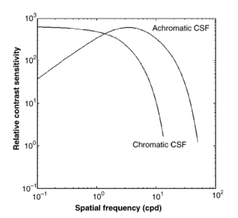
That was news to me. I’d always thought that the emphasis that the Bayer array placed on green as a proxy for luminance was because human eyes are more sensitive to high-spatial frequency variations in luminance than they are to high-spatial frequency variations in chromaticity:

lum chrom vs freq

I posted my contention that the Bayer array’s oversampling of green was based on the way the eye worked, and the poster asked rhetorically how the eye got to be that way, implying that it was because the world was that way.

Well, you know me. I can’t let an assertion that seems counterintuitive go untested. I took the scene from the last post:

2611

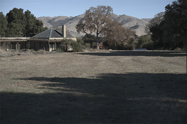
I demosaiced it with AHD in DCRAW, downsampled it to 50% with bicubic sharper, converted it to CIELab, took the 2D Fast Fourier Transform (FFT) of each plane, threw away the phase information by taking the absolute value, squared the result and normalized it by dividing by the product of the number of pixels in each direction. Then I computed a radial average to get a one-dimensional plot with the average of all possible directional power spectra in the image, and plotted that:

radial PSD AHD

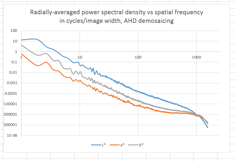
It doesn’t look like the chromaticity is rolling off any faster than the luminance at the highest spatial frequencies. In fact, if anything it’s rolling off a little slower.

I also demosaiced the same raw file with the 2×2 method, and performed the same analysis:

radial PSD 2x2

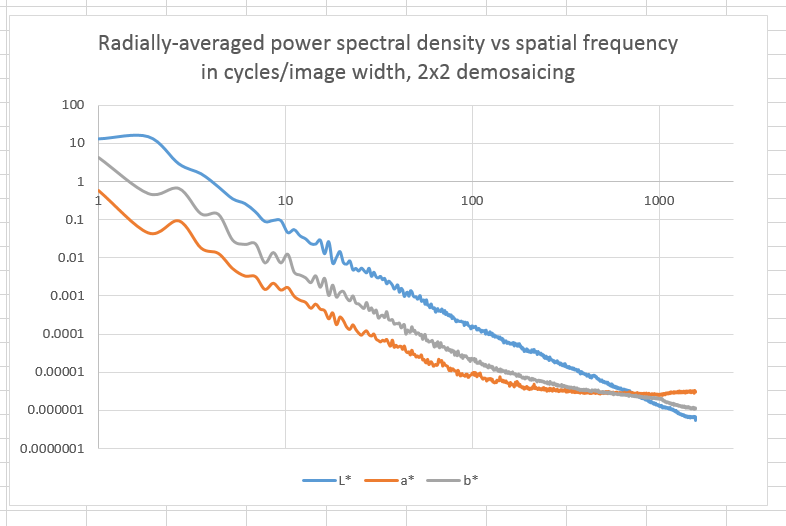
There is even more high-spatial-frequency chromaticity energy now. However, I don’t think that’s real; I think it’s because the 2×2 technique creates more very small chromaticity errors.

That’s only one image. In order to gain some confidence, I’ll have to analyze a few more.

The Last Word

← Color photography without demosaicing in the real world Luminance and chromaticity vs spatial frequency, part 2 →

Leave a Reply Cancel reply

Your email address will not be published. Required fields are marked *

March 2023
S M T W T F S
 1234
567891011
12131415161718
19202122232425
262728293031  
« Jan    

Articles

  • About
    • Patents and papers about color
    • Who am I?
  • Good 35-70 MF lens
  • How to…
    • Backing up photographic images
    • How to change email providers
  • Lens screening testing
    • Equipment and Software
    • Examples
      • Bad and OK 200-600 at 600
      • Excellent 180-400 zoom
      • Fair 14-30mm zoom
      • Good 100-200 mm MF zoom
      • Good 100-400 zoom
      • Good 100mm lens on P1 P45+
      • Good 120mm MF lens
      • Good 18mm FF lens
      • Good 24-105 mm FF lens
      • Good 24-70 FF zoom
      • Good 35 mm FF lens
      • Good 60 mm lens on IQ3-100
      • Good 63 mm MF lens
      • Good 65 mm FF lens
      • Good 85 mm FF lens
      • Good and bad 25mm FF lenses
      • Good zoom at 24 mm
      • Marginal 18mm lens
      • Marginal 35mm FF lens
      • Mildly problematic 55 mm FF lens
      • OK 16-35mm zoom
      • OK 60mm lens on P1 P45+
      • OK Sony 600mm f/4
      • Pretty good 16-35 FF zoom
      • Pretty good 90mm FF lens
      • Problematic 400 mm FF lens
      • Tilted 20 mm f/1.8 FF lens
      • Tilted 30 mm MF lens
      • Tilted 50 mm FF lens
      • Two 15mm FF lenses
    • Found a problem – now what?
    • Goals for this test
    • Minimum target distances
      • MFT
      • APS-C
      • Full frame
      • Small medium format
    • Printable Siemens Star targets
    • Target size on sensor
      • MFT
      • APS-C
      • Full frame
      • Small medium format
    • Test instructions — postproduction
    • Test instructions — reading the images
    • Test instructions – capture
    • Theory of the test
    • What’s wrong with conventional lens screening?
  • Previsualization heresy
  • Privacy Policy
  • Recommended photographic web sites
  • Using in-camera histograms for ETTR
    • Acknowledgments
    • Why ETTR?
    • Normal in-camera histograms
    • Image processing for in-camera histograms
    • Making the in-camera histogram closely represent the raw histogram
    • Shortcuts to UniWB
    • Preparing for monitor-based UniWB
    • A one-step UniWB procedure
    • The math behind the one-step method
    • Iteration using Newton’s Method

Category List

Recent Comments

  • JimK on Fujifilm GFX 100S pixel shift, visuals
  • Sarmed Mirza on Fujifilm GFX 100S pixel shift, visuals
  • lancej on Two ways to improve the Q2 handling
  • JimK on Sony 135 STF on GFX-50R, sharpness
  • K on Sony 135 STF on GFX-50R, sharpness
  • Mal Paso on Christmas tree light bokeh with the XCD 38V on the X2D
  • Sebastian on More on tilted adapters
  • JimK on On microlens size in the GFX 100 and GFX 50R/S
  • Kyle Krug on On microlens size in the GFX 100 and GFX 50R/S
  • JimK on Hasselblad X2D electronic shutter scan time

Archives

Copyright © 2023 · Daily Dish Pro On Genesis Framework · WordPress · Log in

Unless otherwise noted, all images copyright Jim Kasson.