• site home
  • blog home
  • galleries
  • contact
  • underwater
  • the bleeding edge

the last word

Photography meets digital computer technology. Photography wins -- most of the time.

You are here: Home / The Last Word / Balancing real and fake detail — part 3

Balancing real and fake detail — part 3

February 3, 2020 JimK 5 Comments

This is the third post on balancing real and fake detail in digital images. The series starts here.

In the last post, in this series, I showed you some plots of a real sharpness metric and an aliasing metric versus f-stop for an ideal diffraction-limited lens and a camera with a 3.76 micrometer pixel pitch and a 100% fill factor. To tie this mathematical exercise to the real world, both the Fuji GFX 100 and the Sony a7RIV materially fit that description. Those graphs has two measures, and humans, including this one, are biased to seek scalars. You lose a lot when you go from a vector to a scalar space, and the issue of how to weight the dimensions of the vector is infinitely malleable, but I thought I’d give it a whack here.

My proposed metric is simply the normalized amount of energy below Nyquist (which results in accurate reconstruction) minus the (same normalization) amount of energy above Nyquist, which results in bogus (in this case, at least, bogus is a technical term for erroneous) reconstruction.

Here’s what that looks like for our diffraction-limited lens, with a Bayer-CFA Nyquist frequency divisor of 1.5:


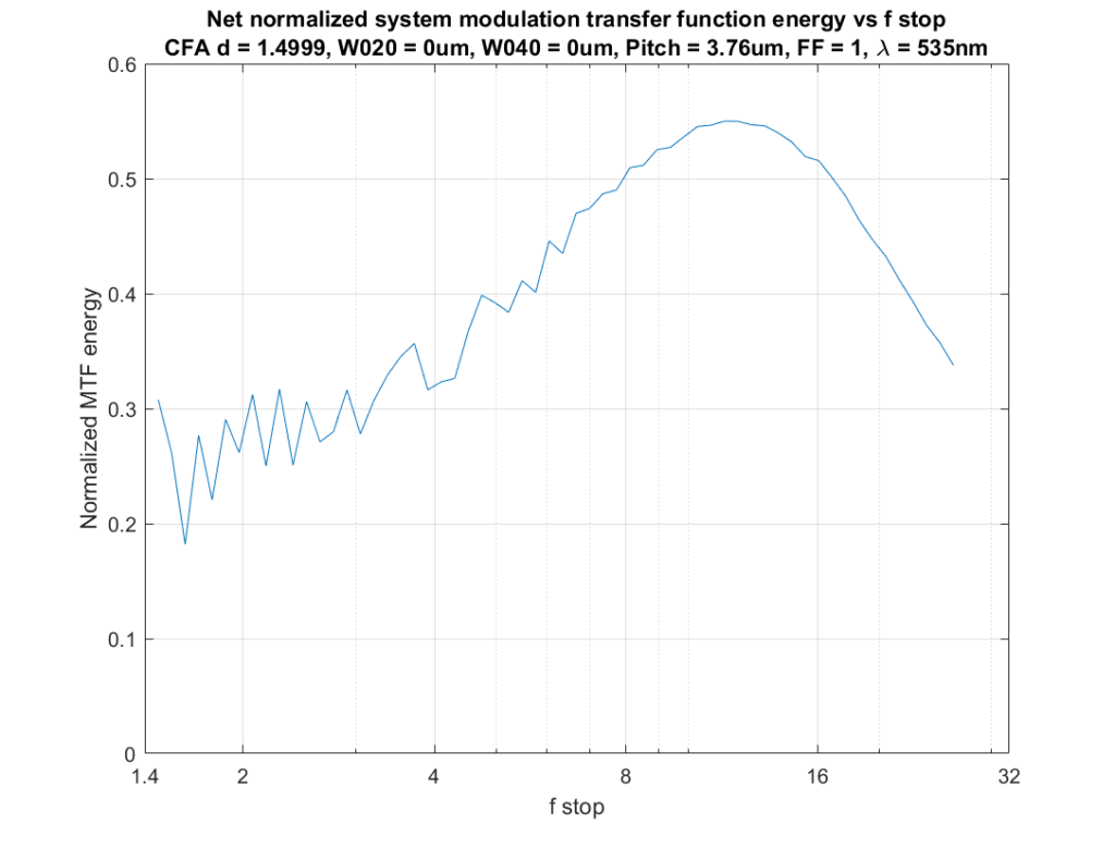
The sweet spot is between f/8 and f/16. That seems like a long way to stop down. Here are some reasons why you might be able to get away with a wider aperture:

  • Your subject doesn’t have a ton of high-frequency detail
  • Your focusing isn’t perfect
  • Your subject is three dimensional
  • Your lens isn’t diffraction limited
  • You and your viewers don’t notice aliased detail much
  • You and your viewers actually like the crisp look that aliasing provides


The Last Word

← Balancing real and fake detail — part 2 Fuji 50/3.5 on GFX 100 →

Comments

  1. Erik Kaffehr says

    February 3, 2020 at 11:05 pm

    Jim,

    It could be interesting if you have rerun some of your calculations with OLP filter.

    I would also much thank you for sharing your knowledge and experience in so many fields related to photography.

    Best regards
    Erik

    Reply
  2. FredD says

    February 5, 2020 at 8:28 am

    Jim, I appreciate your attempt in this series to relate the results predicted to your experience at specific f-stops, (which does certainly validate your analysis as ballpark-correct, at least at these specific pixel sizes), and you do here have a list of caveats. But I couldn’t help but remember an old analysis by Kjell Carlsson of the pinhole camera:

    The Pinhole Camera Revisited
    or
    The Revenge of the Simple-Minded Engineer
    https://www.kth.se/social/files/542d2d2df276546ca71dffaa/Pinhole.pdf

    My point is that the above reminds that not only area under the mtf curve (or parts thereof) but also its shape can be very important in perceived quality. Might apply not only to resolution but also moire analysis.

    So perhaps desirable to weight the mtf values by applying some transformation function that emphasizes human visual system response?

    That said, I’m probably being too picky, and your analysis is much appreciated.

    Reply
    • JimK says

      February 5, 2020 at 8:40 am

      So perhaps desirable to weight the mtf values by applying some transformation function that emphasizes human visual system response?

      Like Ed Granger’s SQF?

      http://www.imatest.com/docs/sqf/

      That requires specifying a print size and viewing distance.

      Reply
      • FredD says

        February 5, 2020 at 9:04 am

        Yes, possibly SQF (though I’m not familiar with alternate ones, so I’d be hard-pressed to know what would be best).

        And while SQF would be at specific print sizes (and distances), once those were decided upon it’s not that difficult in presentation, as a color-coded chart for that was standard at Popular Photography for many years.

        Reply
        • JimK says

          February 5, 2020 at 9:10 am

          And while SQF would be at specific print sizes (and distances), once those were decided upon it’s not that difficult in presentation, as a color-coded chart for that was standard at Popular Photography for many years.

          I’m not eager to write that code.

          Reply

Leave a Reply Cancel reply

Your email address will not be published. Required fields are marked *

May 2025
S M T W T F S
 123
45678910
11121314151617
18192021222324
25262728293031
« Apr    

Articles

  • About
    • Patents and papers about color
    • Who am I?
  • How to…
    • Backing up photographic images
    • How to change email providers
    • How to shoot slanted edge images for me
  • Lens screening testing
    • Equipment and Software
    • Examples
      • Bad and OK 200-600 at 600
      • Excellent 180-400 zoom
      • Fair 14-30mm zoom
      • Good 100-200 mm MF zoom
      • Good 100-400 zoom
      • Good 100mm lens on P1 P45+
      • Good 120mm MF lens
      • Good 18mm FF lens
      • Good 24-105 mm FF lens
      • Good 24-70 FF zoom
      • Good 35 mm FF lens
      • Good 35-70 MF lens
      • Good 60 mm lens on IQ3-100
      • Good 63 mm MF lens
      • Good 65 mm FF lens
      • Good 85 mm FF lens
      • Good and bad 25mm FF lenses
      • Good zoom at 24 mm
      • Marginal 18mm lens
      • Marginal 35mm FF lens
      • Mildly problematic 55 mm FF lens
      • OK 16-35mm zoom
      • OK 60mm lens on P1 P45+
      • OK Sony 600mm f/4
      • Pretty good 16-35 FF zoom
      • Pretty good 90mm FF lens
      • Problematic 400 mm FF lens
      • Tilted 20 mm f/1.8 FF lens
      • Tilted 30 mm MF lens
      • Tilted 50 mm FF lens
      • Two 15mm FF lenses
    • Found a problem – now what?
    • Goals for this test
    • Minimum target distances
      • MFT
      • APS-C
      • Full frame
      • Small medium format
    • Printable Siemens Star targets
    • Target size on sensor
      • MFT
      • APS-C
      • Full frame
      • Small medium format
    • Test instructions — postproduction
    • Test instructions — reading the images
    • Test instructions – capture
    • Theory of the test
    • What’s wrong with conventional lens screening?
  • Previsualization heresy
  • Privacy Policy
  • Recommended photographic web sites
  • Using in-camera histograms for ETTR
    • Acknowledgments
    • Why ETTR?
    • Normal in-camera histograms
    • Image processing for in-camera histograms
    • Making the in-camera histogram closely represent the raw histogram
    • Shortcuts to UniWB
    • Preparing for monitor-based UniWB
    • A one-step UniWB procedure
    • The math behind the one-step method
    • Iteration using Newton’s Method

Category List

Recent Comments

  • bob lozano on The 16-Bit Fallacy: Why More Isn’t Always Better in Medium Format Cameras
  • JimK on Goldilocks and the three flashes
  • DC Wedding Photographer on Goldilocks and the three flashes
  • Wedding Photographer in DC on The 16-Bit Fallacy: Why More Isn’t Always Better in Medium Format Cameras
  • JimK on Fujifilm GFX 100S II precision
  • Renjie Zhu on Fujifilm GFX 100S II precision
  • JimK on Fuji 20-35/4 landscape field curvature at 23mm vs 23/4 GF
  • Ivo de Man on Fuji 20-35/4 landscape field curvature at 23mm vs 23/4 GF
  • JimK on Fuji 20-35/4 landscape field curvature at 23mm vs 23/4 GF
  • JimK on Fuji 20-35/4 landscape field curvature at 23mm vs 23/4 GF

Archives

Copyright © 2025 · Daily Dish Pro On Genesis Framework · WordPress · Log in

Unless otherwise noted, all images copyright Jim Kasson.