I ran the simulated Otus 55mm f/1.4 though the suite of MTF10 tests, and I’ll show the same plats as in the previous post for both a simulated camera with a 4-way beam-splitter anti-aliasing filter and one wit no AA filter.
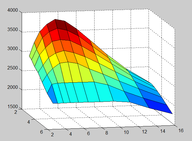
First, the 3 dimensional surface plots.
With no AA filter:
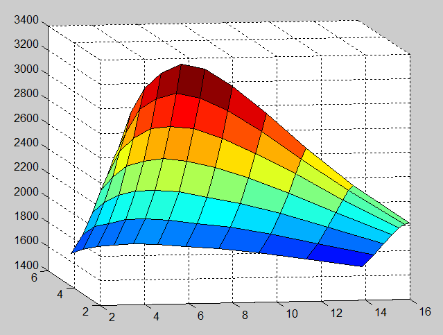
With the AA filter:
Next, contour plots.
With no AA filter:
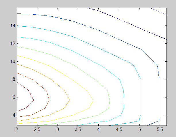
The flat vertical lines on the right hand side are regions where the MTF10 occurs above the Nyquist frequency, and that frequency is substituted.
With the AA filter:
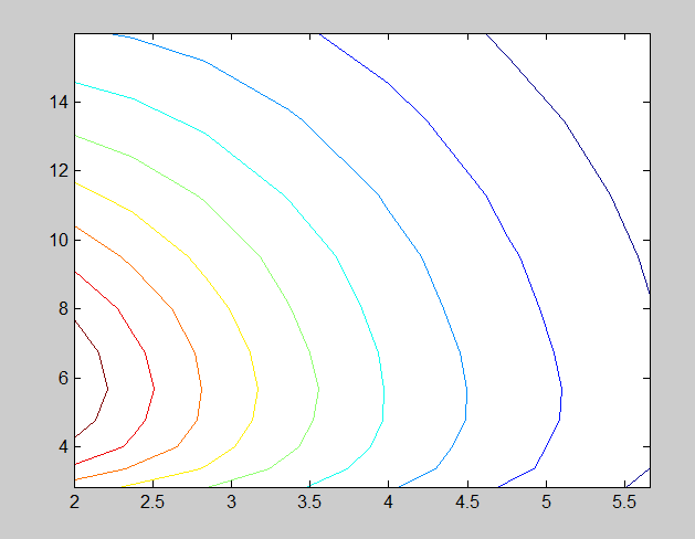
The AA filter insures that MTF10 always occurs below the Nyquist frequency.
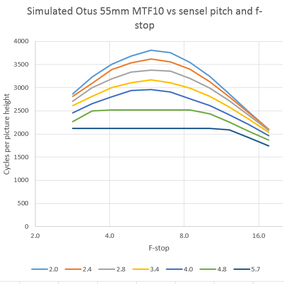
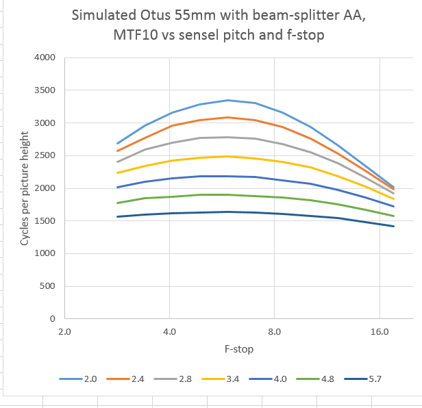
Two dimensional families of curves.
With no AA filter:
With the AA filter:
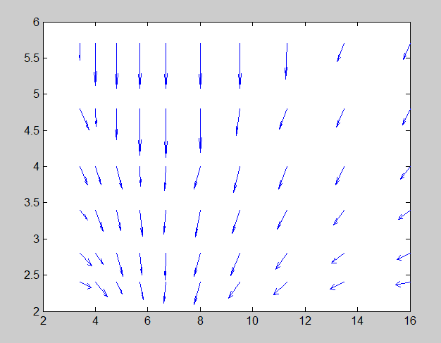
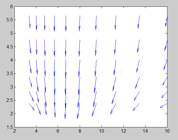
And finally, the quiver plots with the arrows pointing at the direction of steepest ascent (with log-log scaling) and their lengths proportional to the slope in that direction.
With no AA filter:
With the AA filter:
The conclusion: for the simulated Otus, at any stop the most rapid route to greater resolution is in the direction of increased sensel density from those available in full frame cameras today, rather than moving the lens aperture to one with greater resolution.
Leave a Reply