This is part of a series of posts about the Nikon D5. The series starts here.
I completed my first pass at modeling the Nikon D5.There’s a lot more to come, I’m sure. For this first run, I modeled the camera at each tested ISO independent of all the others, and ignored any suspicions that I might have about what’s going on under the hood that’s different from the standard model.
For those of you who are not regular readers, here’s an overview of the protocol.
Jack Hogan and I wrote some Matlab code to analyze pixel response non-uniformity (PRNU), to plot complete photon response curves, and to model sensor behavior. At present, the suite of programs does not analyze dark frame-to-frame persistent patterning, although I have done some of that in the past.
For all the testing except the PRNU, captures are made in pairs. By subtracting a pair of images, a image with 1.414 times the frame-independent noise, unpolluted by static noise, can be obtained, Earlier work did the captures of flat fields; one pair of images was needed for each point of the photon transfer curve (PTC). A PTC plots standard deviation versus mean value, usually using a log scale for both. While using a pair for every data point promoted accuracy, it was truly labor intensive; one set of exposures for each ISO setting for a given camera could number in the mid- thousands.
In order to reduce the number of necessary captures, I created a two-dimensional target. Here is the one that I’m currently using:

You will note the absence of patches in the target. The patches are created by the software sampling the target, and they can be any convenient shape, size, and number. For the results I’m posting here, I used 12 columns and 8 rows of 200×200 pixels. The fact that the target is a gradient is not important for any single patch, since subtracting the two samples takes that out of the picture. It is important to keep the sample extents small enough that most of the sampled values are close together. That must be balanced against wanting many pixels in each sample for the purpose of having solid statistics. As it turns out, with today’s high-resolution cameras, that is no problem.
The capture protocol that I have selected is to make a set of pairs at each camera ISO setting of interest using aperture priority, exposure compensation to get the upper left corner near full scale, and varying the ISO setting. That gets the upper end of the photon transfer curves for each ISO.
I also need a set of exposures nearer, but not at, the black point, which I can use to model the read noise of the camera. To get rid of quantizing artifacts, I have the program throw away samples with SNRs of less than 2, so very dark values are automatically eliminated. If the camera under test were completely ISOless, the same exposure would suffice for each dark capture, no matter what the ISO setting. My hope was that the target would have enough dynamic range so that one exposure setting would suffice even in cameras that significantly depart fro ISOless behavior. So far that has worked out.
I made two sets of dark images, one with a factor of ten (a little over three stops) less exposure than the base ISO aperture priority series, independent of ISO, and one another factor of ten below that.
Here are the D5 measured and modeled values at selected ISOs:
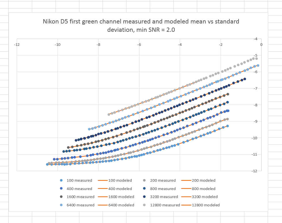
The fit is good.
Here’s what the model has to say about read noise:
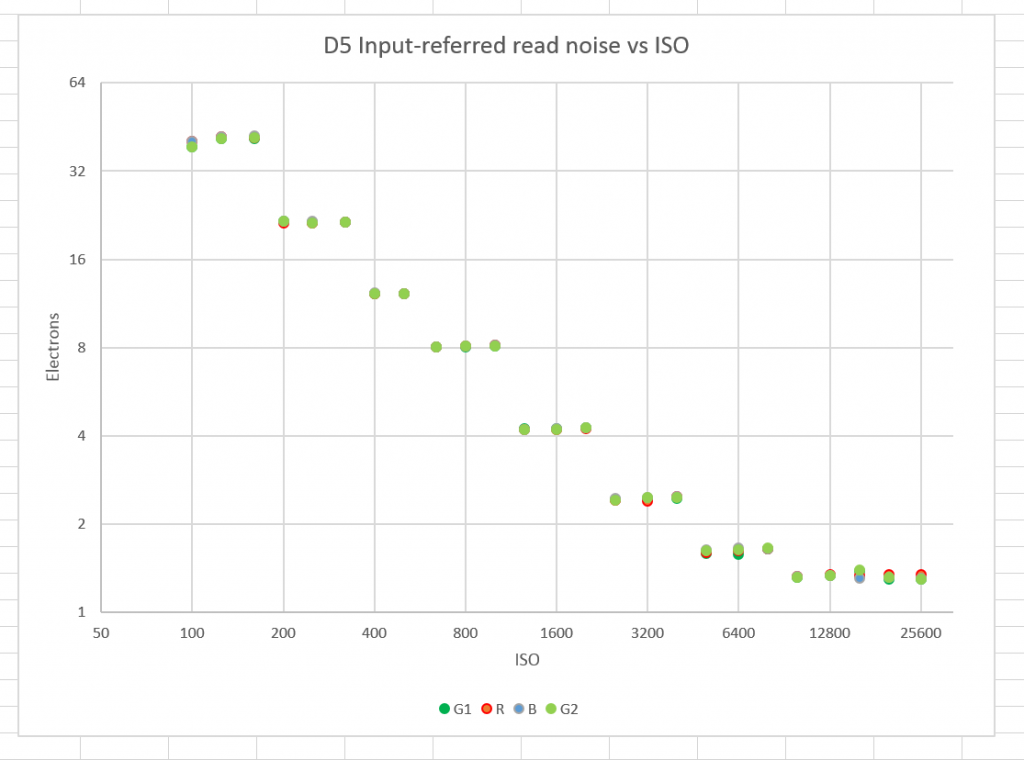
Pretty similar to what we saw before just looking at the dark-field images, but know we know the input referred RN in electrons.
Here is the modeled full well capacity (FWC) versus ISO setting:
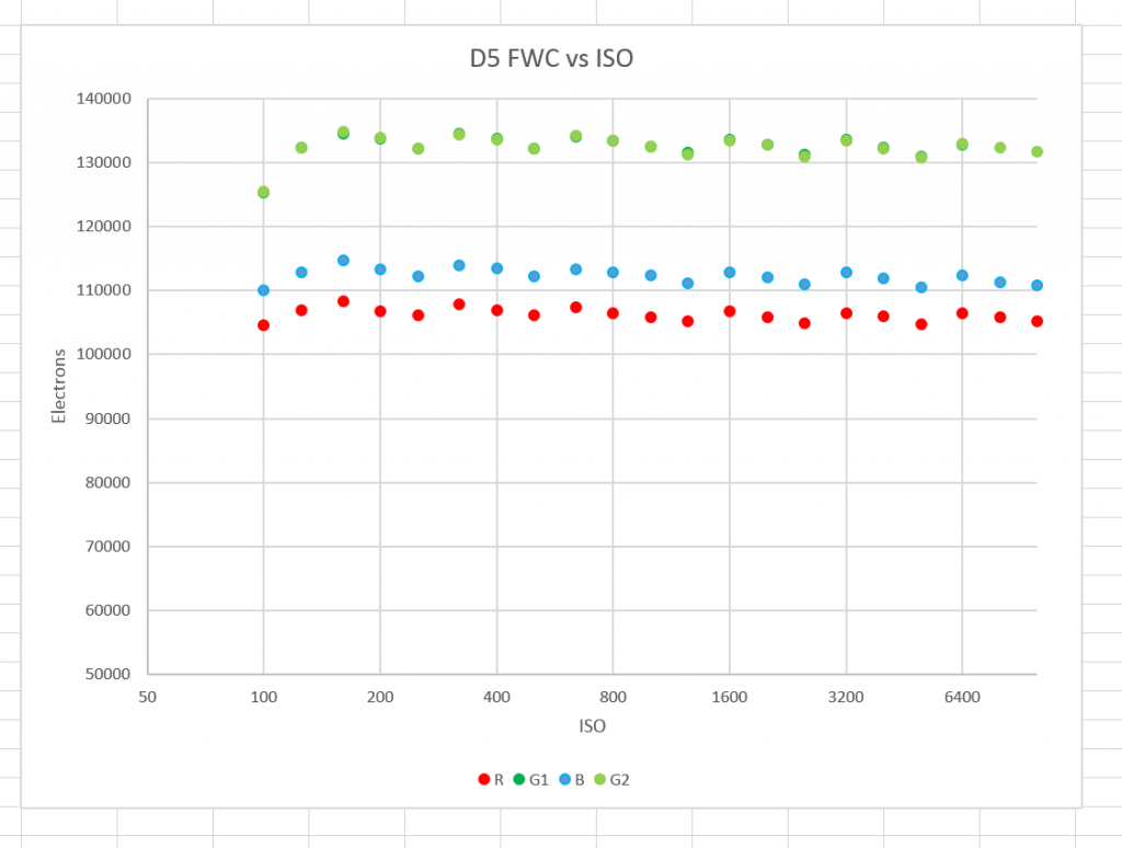
There’s a little sawtooth effect, but it’s well down. We see different values for each class of raw plane, though. Both green planes yield essentially the same numbers, and those are roughly 30% higher than those for the red and blue planes. We’ve seen this before with other Nikon cameras; it appears to have something to do with the white balance prescaling.
I’m going to call the FWC of the D5 130,000 electrons, give or take.
Leave a Reply