This is one in a series of posts on the Fujifilm GFX 100. You should be able to find all the posts about that camera in the Category List on the right sidebar, below the Articles widget. There’s a drop-down menu there that you can use to get to all the posts in this series; just look for “GFX 100”.
Yesterday I looked at the dark-field (read) noise for the GFX 100 using various modes. This morning, I made test images and created photon transfer curves (PTCs) for the camera using 14-bit raw precision and electronic shutter (ES) mode. Using ES made my life easier, since it goes all the was to 1/16000 second, which meant that I didn’t have to use neutral-density filters. I tested the whole-stop ISOs from 100 through 12800. When I’m making the captures, I make pairs of images at each exposure, and during the processing, I subtract them to eliminate any fixed pattern noise, whether low-lever read noise patterning, or pixel response non-uniformity (PRNU), which doesn’t matter much except in bright regions.
I don’t always do PTCs when I test a new camera, and sometimes rely on Bill Claff’s web site for the full-well capacities of the sensor, but I thought it worthwhile to take a morning to do them here, partly because the GFX 100 is an important camera, and partly because it is likely that the 3.76 micrometer (um) pixel used in the GFX 100 is very similar, if not the same as, the same-sized pixels used in the Phase One IQ4 150MP and the Sony a7RIV.
At ISO 100 and 200 in 14-bit precision, the GFX 100 has a black point of 63. At the other ISOs that I used in this test, the black point is 1023. The software that I’ve written to do these kinds of analyses expects the black point to be the same for the whole ISO series, which has been the case with all the cameras that I’ve tested up to now. It would be a pain to rewrite it the right way, making it pick up the black point from the EXIF data, so I’ll show you two sets of curves.
This isn’t the whole PTC, and the vertical axis isn’t the usual rms value of the noise that you find in the traditional PTC. There’s a method to my madness, and this set of curves tells you pretty much all you need to know about the GFX 100’s shadow performance.
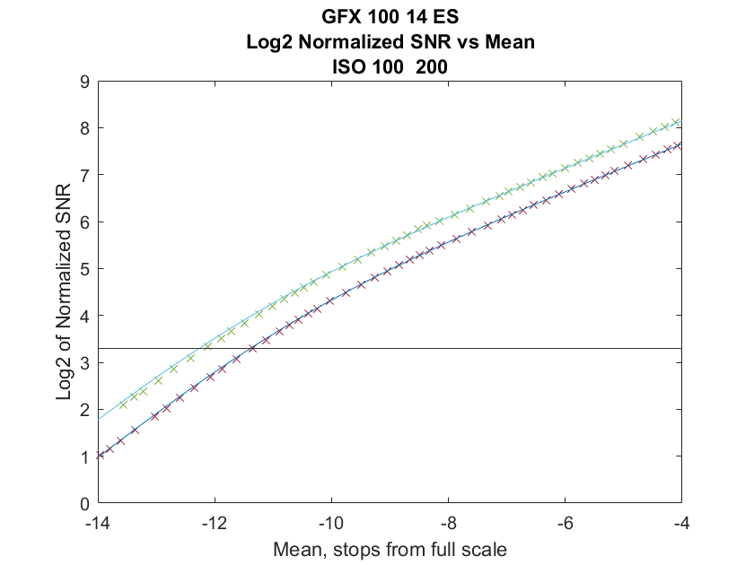
I computed the Photon Transfer Curve (PTC) from the raw files of the camera under test, converted that to signal-to-noise ratio (SNR) vs mean illumination, normalized that for print size and plotted the result. The horizontal black line is significant. This corresponds to an SNR of 10 for an 8-inch high print viewed with a circle of confusion of 1/200 inch, which occurs at a viewing distance of roughly 18 inches for most people with 20/20 vision.
Since most printers have resolutions of 240 to 400 pixels per inch (ppi), to really perform the experiment implied by the metric, you’d have to downsize the image of a modern high-end camera before sending it to the printer. If you used linear methods, that operation performs about the same kind of averaging as the humane eye does, so if you limit yourself in that way, then that part of assumptions is reasonable. It is less reasonable with modern cameras and printers that an 8-inch high print would be the final form of a capture. If that were the case, there would be no reason to purchase cameras with more that about 4 mega-pixels of resolution. However, if you want to raise the bar to an SNR of 10 with a 16-inch high print, all you have to do is move the horizontal line up a bit over 3 units.
The horizontal axis is the average signal level relative to full scale for the camera.
The top set of crosses and lines is for ISO 100, and the bottom set is for ISO 200. The x’s are the measured values, and the continuous lines are the ones that I’ve modeled. They are in excellent agreement except that for very dark areas at ISO 100, where the modeled camera is slightly noisier than the actual one. Looking at where the ISO 100 line crosses the horizontal black line shows that the Claff Photographic Dynamic Range of the GFX 100 at base ISO is about 12.5 stops.
Here are the curves for the other ISO settings that I tested.
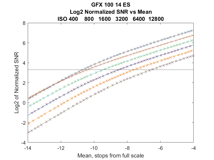
The top line on the right is ISO 400, and the rest are 800,1600, 3200, 6400, and 12800, proceeding downward. Because the GFX 100 increases the conversion gain at the transition from ISO 400 to ISO 500, the read noise crops there. In fact, it drops enough that below about 10 stops down from full scale, ISO 800 is no more noisy than ISO 400.
Now let’s drop the normalization, and zoom out to look at the whole curve for ISO 100.
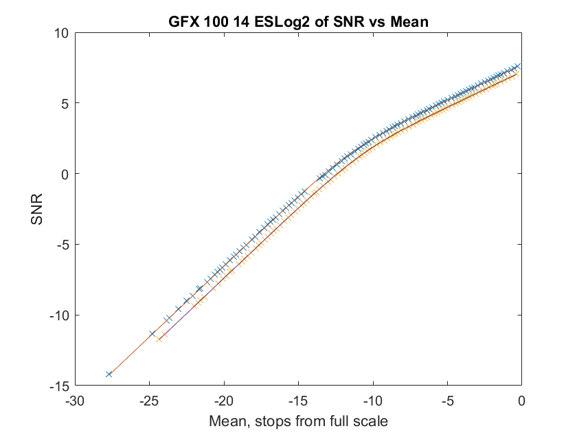
When I do this, I’m looking for anomalies that indicate that the 14-bit precision that I used is insufficient. I’m seeing none of those, so it looks like the read noise of the camera is enough to dither the analog to digital converter properly, and switching to 16-bit precision will probably provide no benefit. I’ll be checking that visually later on.
The modeling that I do provides the camera’s full well capacity (FWC) and read noise. Having both allows the calculation of the read noise in electrons in the photodiode of the sensor, assuming a perfect signal chain from then on; this is called input-referred read noise.
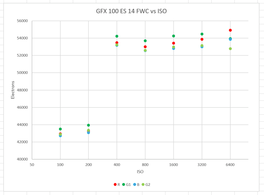
I performed the FWC calculation at each ISO setting, and refered it back to the FWC at base ISO. This is a test of the accuracy of the model, and all the values should be the same. It is clear that the ISO 100 and ISO 200 FWC’s while consistent among the four raw channels, are out of whack with the FWC’s computed with the samples from the higher ISOs. I don’t know why this is the case. I am suspicious that it has to do with in-camera raw processing, since the two ISOs that show abnormally low FWCs are the two that use different black points.
I have been expecting the GFX 100 FWC to come in around 50000 electrons. It looks like on average, I was about right, but that doesn’t make me completely comfortable with the situation.
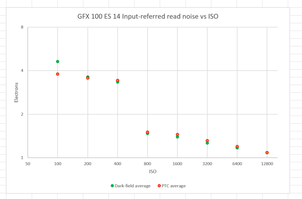
Using the FWCs computed by the modeler, we can compare the read noise that I measured with dark-field images with that implied by the PTCs:
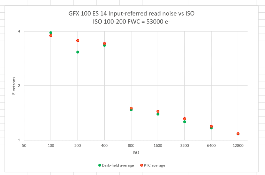
If I arbitrarily make the FWC at ISO 100 and 200 53000 electrons, we get this:
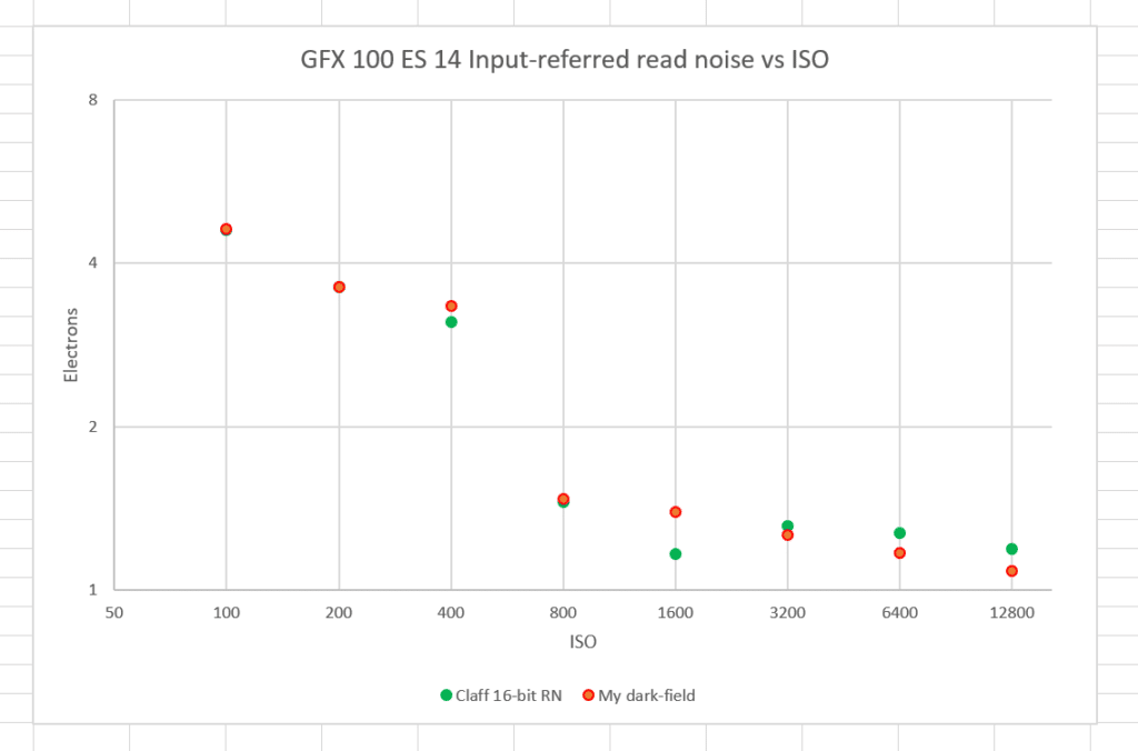
If we compare Bill’s read noise (using my FWCs) with mine dark-field measurements, we find them much the same:
Leave a Reply